Weir Equations in HEC-RAS

Written by Christopher Goodell, P.E., D.WRE
Copyright © The RAS Solution 2016.  All rights reserved. 

HEC-RAS has the ability to simulate flow at hydraulic controls in a variety of ways.  

Bridges, culverts, inline structures, lateral structures, and SA/2D area connections can all act as hydraulic controls.  Effectively, they break up the conservation equations used between cross sections in a 1D reach and/or cells in a 2D area with empirically derived (and usually very stable!) equations.  Weir equations can be used to define flow over an obstruction and are available with all of the 5 hydraulic controls identified above.  However, there are a number of options to consider when selecting simulating weir flow in HEC-RAS.  HEC-RAS approaches weir flow with three different cases:  Ungated Inline Weirs, Ungated Lateral Weirs, and Gated Weirs.  They all begin with the same standard equation:

                                                                  (1)

Where:  Q = discharge, C =weir coefficient, L = weir crest length, H = Energy head over the weir crest.

But each of the three cases apply the weir equation slightly differently. 

Before I continue, I should discuss the difference between the weir coefficient and the discharge coefficient.  I see both of them used interchangeably, but they ARE different.  The weir coefficient (as shown above in the weir equation) is a lumped parameter that includes the discharge coefficient, the gravitational constant, and constants based on geometric properties. 

                                                                                   

                                                                                                                              (2)

Where Cd is the discharge coefficient.  

The discharge coefficient is dimensionless and therefore it is the same in both English (U.S. Customary) Units and SI Units.  The weir coefficient, since it is a function of the gravitational constant, is not dimensionless and therefore has different values depending on which unit system you are using.  For example, a weir coefficient (C) of 3.00 in English Units would be 1.66 in SI units.  But both share the same discharge coefficient (Cd) of 0.56.  For convenience, to convert an English weir coefficient to an equivalent SI weir coefficient, multiply the English weir coefficient by 0.552.  

Be very cautious when considering C versus Cd.  They are different but are often mistakenly used interchangeably.  In fact, you’ll see the coefficient Cd labeled occasionally in the HEC-RAS software and literature when discussing weir coefficient. 

Ungated Inline Weirs. 

When defining inline flow over an “ungated” obstruction (bridge, culvert embankment, inline structure, SA/2D area connection), you have two options for computing weir flow:  Broad Crested and Ogee.   

Figure 1.  Inline structure weir embankment editor.

Both use the same standard weir equation presented above in equation (1).

The only difference between the Broad Crested Option and the Ogee Option is that for the Broad Crested option, the user enters a weir coefficient for C.  For the Ogee option, the user enters a spillway approach height and the ogee’s design energy head, and HEC-RAS will compute the weir coefficient for you.  This may sound convenient, but as the name implies, this option should really be used only for ogee-shaped spillways.  And you would have to know what the design energy head is, a design parameter that is not usually easy to come by, unless you have the hydraulic design report for the spillway.  With both options, submergence reduction of the discharge is automatically calculated with their own respective methods (FHWA ,1978 for broad crested, and COE, 1965 for ogee).

Ungated Lateral Weirs.

Lateral weirs are entered in the lateral structure editor.  Inside the lateral structure’s weir embankment editor, you’ll see two options for weir computations:  Standard Weir Eqn. and Hager’s Eqn.

Figure 2.  Lateral Weir Embankment Editor.

In version 5.0.1, the Standard Weir Eqn. provides four options for the weir crest shape:  Broad Crested, Ogee, Sharp Crested, and Zero Height.  Caution!  Zero Height is NOT used when Standard Weir Eqn. is selected.  This is a bug and will most likely be fixed for future versions.  If you do select Zero Height and Standard Weir Eqn. together, HEC-RAS will just use the weir coefficient you provide with the broad crested methodology.  Sharp Crested is not fully functional in Lateral Structures for version 5.0.1.  You’ll notice that no additional input options (like Rehbock and Kindsvater-Carter, as discussed under the next section, “Gated Weirs) are available when you select Sharp Crested in the lateral weir embankment editor.  My guess is that if you select Sharp Crested, it too will default to the broad crested methodology. 

Broad Crested and Ogee work the same as with the ungated inline structures.

With Hager’s Equation, all four weir crest shapes are available, including the zero-height weir.  The same weir equation is used, but an adjusted weir coefficient is computed based on physical and hydraulic properties.  Each of the four weir types has its own method for computing the adjusted weir coefficient.  There is an input box for “default weir coefficient”.  This is only used for the first iteration of solving Hager’s Equation.  Since Hager is a function of hydraulic properties, it must be solved in an iterative fashion.  After the first iteration, the adjusted weir coefficient will be computed and used.  Page 8-18 of the Hydraulic reference manual discusses Hager’s equation and how the adjusted weir coefficient is computed. 

Zero-height weirs are used for cases where flow will leave a channel laterally, but there is no defined obstruction or hydraulic control separating the two.  Commonly this is used to simulate flow from a main channel up a tributary that is being modeled using a lateral structure and a storage or 2D area.  The HEC-RAS 2D manual has a table of lateral weir coefficients (Table 1). 

Table 1.  Lateral Weir Coefficients (from the HEC-RAS 2D Manual, page 3-50).

Notice the last category is “non elevated” overbank terrain.  If you wish to use the weir coefficients in this table to simulate a non-elevated weir, do not use the Zero-Height weir.  That is strictly for Hager’s equation and Hager’s method automatically computes the weir coefficient.  Instead, use the broad crested standard equation and enter in the non-elevated weir coefficient there. 

Gated Weirs. 

When modeling gated spillways at inline structures or lateral structures, users can provide a weir coefficient for flow over the spillway when the gate is completely opened, and out of contact with the flow (Figure 3). This is different from the discharge coefficient used for flow over the top of the inline structure (Figure 1). 

Figure 3. Inline Gate Editor

With gated spillways, the user has three options for the weir shape:  Broad Crested, Sharp Crested, and Ogee (Figure 4).  Broad Crested and Ogee work the same as previously discussed.  The Sharp Crested option also uses the standard weir equation but gives you three options for determining the discharge coefficient:  user-entered, compute with the Rehbock equation, or compute with the Kindsvater-Carter equation.  For both the Rehbock and Kinsvater-Carter methods, the weir coefficient will be computed independently at each time step. So you can have a varying discharge coefficient for varying heads. 

Figure 4.  Inline Gate Editor.

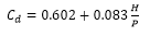
The Rehbock equation for the discharge coefficient was developed for rectangular weirs and is as follows:

                                                                                                                 (3)

Where P = Spillway approach height.  This value must be entered to use the Rehbock equation.  HEC-RAS will then compute the weir coefficient, C using equation (2).   According to Ippen (1950), this equation holds up well for values of H/P up to 5.  And it performs with fair approximation for H/P values up to 10. 

The Kindsvater-Carter method was developed in English units only and is as follows:

                                                                                                        (4)

Where C_e = effective weir coefficient, ft^1/2/s

                k_b = a correction factor to obtain effective weir crest length, ft

            k_h = a correction factor with a constant value of 0.003 ft

The effective weir coefficient, Ce is a function of two ratios:  L/B and H/P, 

Where  L = Weir crest length

            B = Average width of the approach channel

            H = Energy head over the weir crest

            P = Spillway approach height

C_e is a function of both the relative width and relative depth of the approach channel and is taken from the following chart (note that the chart uses the variable h1 for H.  They are the same):

Figure 5.  Effective Weir Coefficient

k_b is used to determine the effective length of the weir crest and is a function of the relative width of the approach channel.  It is taken from the following chart:

Figure 6.  Correction factor k_b.

To use the Kindsvater-Carter method in HEC-RAS for a gated spillway, first select the weir shape as “Sharp Crested”.  Then select “Compute with Kinsvater-Carter eqn as the Weir Method.  You must then choose a relative approach channel width (L/b) and enter the spillway approach height, P (note, b is used in the HEC-RAS Inline Gate Editor for B.  They are the same). 

Figure 7.  Kindsvater-Carter Weir Method.

Remember, the Kindsvater-Carter equation was developed and is presented here in English units.  When using SI units, HEC-RAS will automatically convert the units appropriately.  So you can still enter a spillway approach height in meters if you are using SI units. 

The Kindsvater-Carter weir equation is built for rectangular weirs and “is particularly useful for installations where full crest contractions or full end contractions are difficult to achieve.”  (USBR 2001)  More information on the Kindsvater-Carter equation, including its limitations, can be found here:  http://www.usbr.gov/tsc/techreferences/mands/wmm/chap07_06.html

References:

Federal Highway Administration (FHWA), 1978.  Hydraulics of Bridge Waterways, Hydraulic Design Series No. 1, by Joseph N. Bradley, U.S. Department of Transportation, Second Edition, revised March 1978, Washington D.C.

Ippen, A.T. ,1950.  Channel Transitions and Controls, Chap. VIII in Hunter Rouse (editor): Engineering Hydraulics,” John Wiley & Sons, Inc., New York.  pp.496-588.

Unites State Bureau of Reclamation (USBR), 2001.  Water Measurement Manual, http://www.usbr.gov/tsc/techreferences/mands/wmm/

U.S. Army Corps of Engineers (COE), 1965.  Hydraulic Design of Spillways, EM 1110-2-1603, Plate 33.

Lateral Structure Coefficients

Written by Chris Goodell, P.E., D.WRE  |  WEST Consultants

Copyright © RASModel.com.  2013.  All rights reserved.

Lateral structures can be used in HEC-RAS to transfer flow from a river/reach to a storage area, or to another river/reach.  With the coming release of HEC-RAS with 2D capabilities (estimated beta release January/February 2014), you’ll be able to hook a river/reach to a 2-D area using a lateral structure. 
Although its primary function in HEC-RAS is to transfer flow out of one river/reach into another component (river/reach, storage area, 2D area), a lateral structure can physically represent a wide range of geometric features, including a levee, a flow diversion structure, a morning glory spillway, or even a natural ground or bathymetric profile.  Including a lateral structure in your model to represent a levee is important if the levee is ever overtopped or breached during the simulation.  Flow diversion structures can have multiple outlet features, including culverts, gates, and spillways.  These features are all available in the lateral structure editor in HEC-RAS. 
Another common use of lateral structures is to simulate flow transfer from the river to a tributary during a flood event.  This is especially convenient if you don’t want to model the tributary as an individual reach, but still want to account for it’s available storage, for a proper accounting of flood wave attenuation in the main stem river/reach.  As an example, the following figure shows a storage area representing a tributary to the main stem river.  This storage area is connected to the main stem by a lateral structure (highlighted in red). 

Because a lateral structure can represent a variety of different flow transferring structures (or non-structures), the hydraulics in and around the lateral structure can be quite different, depending upon the case.  Every lateral structure in HEC-RAS requires a lateral weir coefficient, and different hydraulics mean different lateral weir coefficients.  Any hydraulics textbook will have a multitude of weir coefficients for “inline” conditions, but it’s rare to find something similar for lateral flows, or diversion flows.  But it is generally agreed that lateral structure weir coefficients should be much lower than a similar inline configuration.  For example, an inline, hydraulically efficient broad-crested weir might have a weir coefficient around 3.0 (US units) or 1.7 (SI Units).  Turn that structure sideways (a lateral structure), and it will have a coefficient closer to 2.0 (US Units) or 1.1 (SI Units).  The difference is due to the energy/momentum loss associated with turning flow lines from their downstream orientation to a lateral direction out of the river/reach.    Unfortunately, there has simply not been a lot of research done on quantifying this energy/momentum loss and what that does to lateral weir coefficients.
The research that is available could be useful and might be worth checking out.  Hagar’s equation is one reference and is actually built into the HEC-RAS lateral structure editor, under Lateral Weir Embankment…Weir Computations.  It will compute an equivalent lateral weir coefficient based on an inline value (the Default Weir Coefficient) and some physical and hydraulic properties of the weir and  the adjacent river/reach. 

You can read more about Hagar’s equation in the HEC-RAS Hydraulic Reference Manual on page 8-17. 
Useful references for lateral structure weir coefficients (including Hager’s):

• Hager, W.H. (1987). “Lateral Outflow over Side Weirs.” Journal of Hydraulic Engineering, ASCE, 113(4).
• Borghei, S.M.; Malili, M.R.; Ghodsian, M. (1999). “Discharge Coefficient for Sharp-Crested Side Weir in Subcritical Flow.” Journal of Hydraulic Engineering, ASCE, October, 1999.
• Ranga Raju, K.G.; Prasad, B.; Gupta, S.K. (1979). “Side Weir in Rectangular Channel.” Journal of Hydraulic Engineering, ASCE, 105(5).
• Subramanya, K.; Awasthy, S.C. (1972). “Spatially Varied Flow over Side Weirs.” J. Hydr. Div., ASCE, 98(1).
• Singh, R.; Manivannan, D.; Satyanarayana T. (1994). “Discharge Coefficient of Rectangular Side Weirs.” Journal of Irrigation and Drainage Engineering, ASCE, 120(4).

However, none of these references discuss lateral weir coefficients for lateral flow transfers over natural ground, or surface flow (i.e. non-elevation overbank terrain).  HEC has a reference table for lateral structure coefficients that I like to use-it’s also included in the new “Combined 1D and 2D Modeling with HEC-RAS” document that was released in August 2013, in anticipation of the new 2D feature in HEC-RAS expected to be released as a beta version in the January/February 2014 time frame.   Note how low the suggested range of coefficients is for “non-elevated overbank terrain.”  Because they are not dimensionless, be aware that weir coefficients in SI Units are different from US units by a factor of the square root of the ratio of the SI gravitational constant to the US gravitational constant,

What is being modeled with the Lateral Structure	Description	Range of Weir Coefficients
Levee/Roadway – 3 ft (1 meter) or higher above natural ground	Broad crested weir shape, flow over Levee/road acts like weir flow	US Units: 1.5 to 2.2 (2.0 default) SI Units:  0.83 to 1.2 (1.1 default)
Levee/Roadway – 1 to 3 ft (0.3 to 1.0 meter) elevated above ground	Broad crested weir shape, flow over levee/road acts like weir flow, but becomes submerged easily.	US Units:  1.0 to 2.0 SI Units:  0.55 to 1.1
Natural high ground barrier – 1 to 3 ft (0.3 to 1.0 meter) high.	Does not really act like a weir, but must flow over high ground to get into 2D (or storage) area.	US Units: 0.5 to 1.0 SI Units: 0.28 to 0.55
Non-elevated overbank terrain. Lateral Structure not elevated above ground	Overland flow escaping the main river.	US Units: 0.1 to 0.5 SI Units:  0.06 to 0.28

*Hydrologic Engineering Center, August 2013.  “Combined 1D and 2D Modeling with HEC-RAS”

Although this table is presented within the context of 1-D to 2-D flow transfers, these values will work with river/reach to storage area or river/reach to river/reach flow transfers as well.  As noted in the referenced document (HEC 2013), “In general, Lateral Structure weir coefficients should be lower than typical values used for inline weirs.  Additionally, when a lateral structure (i.e. weir equation) is being used to transfer flow from the river (1D region) to the floodplain (2D Flow Area), and then [sic] the weir coefficients that are used need to be very low, or too much flow will be transferred.”  Also, “The number 1 problem people have been having with interfacing 1D river reaches with 2D areas, is user’s [sic] have been using way to [sic] high of weir coefficients for the situation being modeled.  If the lateral structure is really just an overland flow interface between the 1D river and the 2D floodplain, then weir coefficients in the range of 0.1 to 0.5 must be used to get the right flow transfer and keep the model stable.” 

The HEC 2013 document ("Combined 1D and 2D Modeling with HEC-RAS") with the Table of lateral weir coefficients can be downloaded from my Google Drive site here:  https://drive.google.com/file/d/0B_s8OLJOgOi0Nm5sdHFhSzFUYkk/edit?usp=sharing.  The lateral weir coefficient table is on page 35.

Flow spike after peak of dam breach floodwave.

Written by Chris Goodell, P.E., D. WRE | WEST Consultants
Copyright © RASModel.com. 2012. All rights reserved.

Just ran into an interesting phenomenon.  I was running a dam breach model with fairly typical breach parameters and piping failure mode.  After the peak of the breach hydrograph, there appeared a mysterious “spike” as shown in the figure below. 

This happens to be right at the same time the flow through the developing breach becomes freeflowing (as opposed to pressure flow through the breach opening) as shown in the next two figures.


This is the point at which RAS switches from using the orifice equation to the weir equation.  The breach editor allows you to specify a breach weir coefficient.  By lowering this weir coefficient, you can get rid of the spike and have a smoother hydrograph.  I'm not concluding that this spike is incorrect. In fact, it is quite possible that you do experience a real surge when the breach collapses in and goes freeflowing.  In that case, you may find the spike acceptable.  Whichever result you use, be sure you can back it up with sound reasoning.  Given the extreme uncertainty in both breach weir coefficients and piping coefficients, it's probably best that you run a sensitivity analysis to gain a full understanding ot the effects these coefficients have on the dam breach hydrograph. 


Breach weir coefficient = 3.0

Breach weir coefficient = 2.0

Breach weir coefficient = 1.0

Looks like a breach weir coefficient of 1.0 does the trick.