
Written by Chris Goodell, P.E., D.WRE | WEST Consultants
Although its primary function in HEC-RAS is to transfer flow out of one river/reach into another component (river/reach, storage area, 2D area), a lateral structure can physically represent a wide range of geometric features, including a levee, a flow diversion structure, a morning glory spillway, or even a natural ground or bathymetric profile. Including a lateral structure in your model to represent a levee is important if the levee is ever overtopped or breached during the simulation. Flow diversion structures can have multiple outlet features, including culverts, gates, and spillways. These features are all available in the lateral structure editor in HEC-RAS.
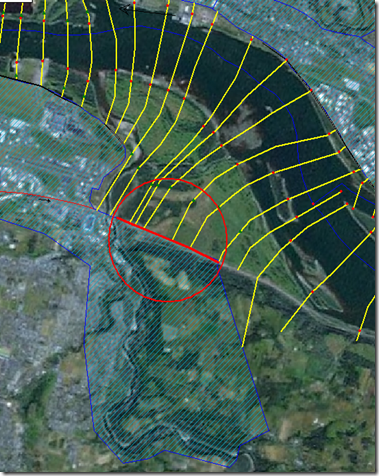
Another common use of lateral structures is to simulate flow transfer from the river to a tributary during a flood event. This is especially convenient if you don’t want to model the tributary as an individual reach, but still want to account for it’s available storage, for a proper accounting of flood wave attenuation in the main stem river/reach. As an example, the following figure shows a storage area representing a tributary to the main stem river. This storage area is connected to the main stem by a lateral structure (highlighted in red).
Because a lateral structure can represent a variety of different flow transferring structures (or non-structures), the hydraulics in and around the lateral structure can be quite different, depending upon the case. Every lateral structure in HEC-RAS requires a lateral weir coefficient, and different hydraulics mean different lateral weir coefficients. Any hydraulics textbook will have a multitude of weir coefficients for “inline” conditions, but it’s rare to find something similar for lateral flows, or diversion flows. But it is generally agreed that lateral structure weir coefficients should be much lower than a similar inline configuration. For example, an inline, hydraulically efficient broad-crested weir might have a weir coefficient around 3.0 (US units) or 1.7 (SI Units). Turn that structure sideways (a lateral structure), and it will have a coefficient closer to 2.0 (US Units) or 1.1 (SI Units). The difference is due to the energy/momentum loss associated with turning flow lines from their downstream orientation to a lateral direction out of the river/reach. Unfortunately, there has simply not been a lot of research done on quantifying this energy/momentum loss and what that does to lateral weir coefficients.
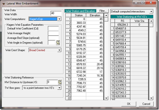
The research that is available could be useful and might be worth checking out. Hagar’s equation is one reference and is actually built into the HEC-RAS lateral structure editor, under Lateral Weir Embankment…Weir Computations. It will compute an equivalent lateral weir coefficient based on an inline value (the Default Weir Coefficient) and some physical and hydraulic properties of the weir and the adjacent river/reach.
You can read more about Hagar’s equation in the HEC-RAS Hydraulic Reference Manual on page 8-17.
Useful references for lateral structure weir coefficients (including Hager’s):
The HEC 2013 document ("Combined 1D and 2D Modeling with HEC-RAS") with the Table of lateral weir coefficients can be downloaded from my Google Drive site here: https://drive.google.com/file/d/0B_s8OLJOgOi0Nm5sdHFhSzFUYkk/edit?usp=sharing. The lateral weir coefficient table is on page 35.
Copyright © RASModel.com. 2013. All rights reserved.
Lateral structures can be used in HEC-RAS to transfer flow from a river/reach to a storage area, or to another river/reach. With the coming release of HEC-RAS with 2D capabilities (estimated beta release January/February 2014), you’ll be able to hook a river/reach to a 2-D area using a lateral structure.Although its primary function in HEC-RAS is to transfer flow out of one river/reach into another component (river/reach, storage area, 2D area), a lateral structure can physically represent a wide range of geometric features, including a levee, a flow diversion structure, a morning glory spillway, or even a natural ground or bathymetric profile. Including a lateral structure in your model to represent a levee is important if the levee is ever overtopped or breached during the simulation. Flow diversion structures can have multiple outlet features, including culverts, gates, and spillways. These features are all available in the lateral structure editor in HEC-RAS.
Another common use of lateral structures is to simulate flow transfer from the river to a tributary during a flood event. This is especially convenient if you don’t want to model the tributary as an individual reach, but still want to account for it’s available storage, for a proper accounting of flood wave attenuation in the main stem river/reach. As an example, the following figure shows a storage area representing a tributary to the main stem river. This storage area is connected to the main stem by a lateral structure (highlighted in red).

Because a lateral structure can represent a variety of different flow transferring structures (or non-structures), the hydraulics in and around the lateral structure can be quite different, depending upon the case. Every lateral structure in HEC-RAS requires a lateral weir coefficient, and different hydraulics mean different lateral weir coefficients. Any hydraulics textbook will have a multitude of weir coefficients for “inline” conditions, but it’s rare to find something similar for lateral flows, or diversion flows. But it is generally agreed that lateral structure weir coefficients should be much lower than a similar inline configuration. For example, an inline, hydraulically efficient broad-crested weir might have a weir coefficient around 3.0 (US units) or 1.7 (SI Units). Turn that structure sideways (a lateral structure), and it will have a coefficient closer to 2.0 (US Units) or 1.1 (SI Units). The difference is due to the energy/momentum loss associated with turning flow lines from their downstream orientation to a lateral direction out of the river/reach. Unfortunately, there has simply not been a lot of research done on quantifying this energy/momentum loss and what that does to lateral weir coefficients.
The research that is available could be useful and might be worth checking out. Hagar’s equation is one reference and is actually built into the HEC-RAS lateral structure editor, under Lateral Weir Embankment…Weir Computations. It will compute an equivalent lateral weir coefficient based on an inline value (the Default Weir Coefficient) and some physical and hydraulic properties of the weir and the adjacent river/reach.

You can read more about Hagar’s equation in the HEC-RAS Hydraulic Reference Manual on page 8-17.
Useful references for lateral structure weir coefficients (including Hager’s):
- Hager, W.H. (1987). “Lateral Outflow over Side Weirs.” Journal of Hydraulic Engineering, ASCE, 113(4).
- Borghei, S.M.; Malili, M.R.; Ghodsian, M. (1999). “Discharge Coefficient for Sharp-Crested Side Weir in Subcritical Flow.” Journal of Hydraulic Engineering, ASCE, October, 1999.
- Ranga Raju, K.G.; Prasad, B.; Gupta, S.K. (1979). “Side Weir in Rectangular Channel.” Journal of Hydraulic Engineering, ASCE, 105(5).
- Subramanya, K.; Awasthy, S.C. (1972). “Spatially Varied Flow over Side Weirs.” J. Hydr. Div., ASCE, 98(1).
- Singh, R.; Manivannan, D.; Satyanarayana T. (1994). “Discharge Coefficient of Rectangular Side Weirs.” Journal of Irrigation and Drainage Engineering, ASCE, 120(4).

| What is being modeled with the Lateral Structure | Description | Range of Weir Coefficients |
| Levee/Roadway – 3 ft (1 meter) or higher above natural ground | Broad crested weir shape, flow over Levee/road acts like weir flow | US Units: 1.5 to 2.2 (2.0 default) SI Units: 0.83 to 1.2 (1.1 default) |
| Levee/Roadway – 1 to 3 ft (0.3 to 1.0 meter) elevated above ground | Broad crested weir shape, flow over levee/road acts like weir flow, but becomes submerged easily. | US Units: 1.0 to 2.0 SI Units: 0.55 to 1.1 |
| Natural high ground barrier – 1 to 3 ft (0.3 to 1.0 meter) high. | Does not really act like a weir, but must flow over high ground to get into 2D (or storage) area. | US Units: 0.5 to 1.0 SI Units: 0.28 to 0.55 |
| Non-elevated overbank terrain. Lateral Structure not elevated above ground | Overland flow escaping the main river. | US Units: 0.1 to 0.5 SI Units: 0.06 to 0.28 |
*Hydrologic Engineering Center, August 2013. “Combined 1D and 2D Modeling with HEC-RAS”
Although this table is presented within the context of 1-D to 2-D flow transfers, these values will work with river/reach to storage area or river/reach to river/reach flow transfers as well. As noted in the referenced document (HEC 2013), “In general, Lateral Structure weir coefficients should be lower than typical values used for inline weirs. Additionally, when a lateral structure (i.e. weir equation) is being used to transfer flow from the river (1D region) to the floodplain (2D Flow Area), and then [sic] the weir coefficients that are used need to be very low, or too much flow will be transferred.” Also, “The number 1 problem people have been having with interfacing 1D river reaches with 2D areas, is user’s [sic] have been using way to [sic] high of weir coefficients for the situation being modeled. If the lateral structure is really just an overland flow interface between the 1D river and the 2D floodplain, then weir coefficients in the range of 0.1 to 0.5 must be used to get the right flow transfer and keep the model stable.”The HEC 2013 document ("Combined 1D and 2D Modeling with HEC-RAS") with the Table of lateral weir coefficients can be downloaded from my Google Drive site here: https://drive.google.com/file/d/0B_s8OLJOgOi0Nm5sdHFhSzFUYkk/edit?usp=sharing. The lateral weir coefficient table is on page 35.


