Pages

Tuesday, December 6, 2016

Time Series Outflows for Dams

Written by Chris Goodell, P.E., D. WRE | WEST Consultants
Copyright © The RAS Solution 2016. All rights reserved.

Want to simulate a time series of outflows for a dam?  It's easy.  In Version 5.0.3 there's a new feature called Outlet T.S. (Outlet Time Series) in the inline structure editor.  


Click the Outlet TS button and give your new time series a name.  You might name it "Powerhouse" or "Fish Bypass" or something like that.  Once you name it and click OK, it seems like nothing happens.  But what you've done is added the ability for the inline structure to have a flow hydrograph assigned to it in the unsteady flow editor.  

Open up the unsteady flow editor and select the "Add RS..." button.  Then select the inline structure to add it to the list of Boundary Conditions.  Notice in this example, I already have a time series of gate openings assigned to this inline structure.  No matter...just add another boundary condition.  If you click on the empty cell next to the inline structure, you'll see that "Flow Hydrograph" is now an available boundary condition type.


Select the Flow Hydrograph button and now you can enter in a time series of flows for whatever feature you are modeling.  


By the way, this new feature is also available for lateral structures.  

Wednesday, November 23, 2016

Resources for 2D Modeling

Now that we've had 2D modeling in HEC-RAS for almost 2 years, I'm curious to know what your favorite 2D Hydraulic Modeling resources are. Of course, for HEC-RAS modeling, the HEC-RAS 2D Manual is excellent, but what about for a more general discussion of 2D Hydraulic Modeling?  Books?  Journal articles?

I like the Australian Rainfall & Runoff Revision Projects, Project 15:  Two Dimensional Modelling in Urban and Rural Floodplains http://arr.ga.gov.au/revision-projects/project-list/projects/project-15

I also like reading the works of Vincenzo Casulli.  Google him.

If you have a favorite resource for 2D modeling, please share it in the comments section below.


Wednesday, October 19, 2016

Creating Static Results Maps (Shapefiles or Rasters) using RAS Mapper

Written by Mikell Warms  |  WEST Consultants
Copyright © The RAS Solution.  2016.  All rights reserved.
Many readers have been asking how to create shapefiles and other static maps in RAS Mapper. One of the main differences between RAS Mapper in RAS 4.1 and RAS 5.0 is the existence of Dynamic Maps. What makes these maps dynamic is that when you have that Results Layer selected in RAS Mapper, you can use the slider bar (top right) to animate through the simulation and see the results of that layer at each mapping output interval (or each profile for steady flow models). These maps are not saved to the disk, they are temporarily stored in memory.


With this change, you can no longer “Export Layer to Shapefile” as you could previously, due to the fact that these dynamic layers are not one map, they are many maps.

To create static maps, such as shapefiles or rasters, we must first tell RAS Mapper what type of static map we want (Inundation Boundary, Velocity, Shear Stress, etc.) and whether we want the data from a specific timestep, or max/min. To do this, right click on the bold “Results” heading in the Layer Manager in RAS Mapper, then choose “Manage Results Maps”.  All of your plans and default layers will load (like below):


Choose the plan you are interested in, and click on “Add New Map.”

If you’re running a Steady model, the window that pops up will look like this: 

If you’re running an Unsteady model, the window that pops up will look like this: 

Choose the Map Type you are interested in creating; in this case we are creating a maximum Inundation Boundary. Notice we have chosen “Maximum” under the Unsteady Profile options, but we could have chosen “Minimum” or a specific point in time. On the right hand side of the window, make sure to change the Map Output Mode to one of the “Stored (saved to disk)” options, depending on your needs. In this case, we are creating a shapefile polygon. Then click Add Map.

One last step. The Manage Results Maps layer should now look like below:


Notice the static map we have added has appeared. However, the Inundation Boundary map status says “Map Not Created”. You will need to select that map, and click on “Compute/Update Stored Maps” at the top right. If you have multiple static maps, you can select them all by holding the CTRL key and selecting multiple maps prior to computing them.

Once the computations have completed, the status will change to “Map files up to date” and RAS will save your shapefile in your HEC-RAS project folder, in a subfolder that has the same name as the plan from which the shapefiles were created.


Thursday, October 13, 2016

Mississippi River Basin Model Clean-Up Day

For all the HEC-RAS users in the Mississippi area, please consider participating in this service event.  A great opportunity to network with others interested in hydraulic models and to help with the restoration of the historic Mississippi River Basin Physical Model.

Please contact Ms. Sarah McEwan at friendsofMRBM@gmail.com or visit https://www.facebook.com/FriendsofMississippiRiverBasinModel
http://www.friendsofmrbm.org/


Wednesday, October 5, 2016

HEC-RAS Version 5.0.3 has been released!

Version 5.0.3 is now available from the HEC website.  Besides bug fixes, there are a few new or improved features of note:  
  • Culvert Inlet/Outlet Control
  • Using 2D Flow Equations at Lateral Structures
  • Flow and Volume Time Series Output on Profile Lines in RAS Mapper
  • Profile Line Point and Tick Marks
  • Legend for RAS Mapper
  • Improvements to sloping and hybrid map rendering modes
Please read the release notes for more information.

Version 5.0.3 can be downloaded here:


Good luck and enjoy!

Tuesday, October 4, 2016

HEC-RAS 5 2D Course in Barcelona / Curso de Modelación Bidimensional con HEC-RAS 5 en Barcelona

Para los compañeros usuarios de HEC-RAS hispanohablantes, mi colega Marty Teal estará dictando nuestro curso de modelación bidimensional con HEC-RAS 5 en español en Barcelona el 19-21 de octubre, solo queda esta semana para inscribirse.

Vaya aquí para más información.

For my fellow Spanish speaking HEC-RAS Users, my colleague Marty Teal will be teaching our HEC-RAS 5 2D Course in Spanish October 19-21 in Barcelona, Spain. 

Go here for more information.

Tuesday, September 27, 2016

Wormhole Culverts

This is one of the coolest workaround ideas for HEC-RAS that I've seen in a long time.  One of my joys in teaching HEC-RAS to professionals and students around the world is seeing the clever ways that people use and apply HEC-RAS.  Whether in a training class, giving technical support, or just simply over discussions with other HEC-RAS users, I still learn new ways to use HEC-RAS almost daily.  However, "Wormhole Culverts" has to be right up near the top of ingenious workarounds.

One current limitation in HEC-RAS 5 is that when you put a culvert or gate in a 2D Area Connection, flow through the culvert or gate can only go from a cell adjacent to the 2D Area Connection line on the upstream side to a cell adjacent to the 2D Area Connection on the downstream side.  If your cell size is relatively small and your culvert is relatively long, then your culvert may in reality span many cells between its upstream side and downstream side.  But the current limitation doesn't allow this.

wormhole_method_culvert_resultsBut we're in luck!  Mr. Con Katsoulas, a senior water resources engineering from SMEC in Sydney Australia came up with a method to get around this limitation.  He first discussed this in The RAS Solution forum.  And my friend and colleague, Mr. Krey Price of Surface Water Solutions wrote a detailed explanation on how to use this technique. Please read his blog post on wormhole culverts for the full description.

Good luck!  Give it a try and let me know how it works for you.

Wednesday, September 21, 2016

HEC-RAS Dam Breach course in New Zealand!

Limited-time early-bird discounts available

Registrations are now available for our dam breach course in Auckland, New Zealand to be held from 29 November to 1 December 2016.  I will be teaching this course with help from Mr. Krey Price of Surface Water Solutions.  Please come and join us!

We have fewer than ten places remaining, so please register soon to confirm your place!
A $250 early-bird discount is available using coupon code “earlybird” at checkout.
Our agenda will cover unsteady flow, level pool versus dynamic routing, breach parameters, setting up a dam breach model, diagnosing and fixing dam breach models, and presentation of 1D and 2D case studies. Hope to see you there! 

Wednesday, September 14, 2016

HEC-RAS 2D Course in Concepcion, Chile November 8-10, 2016

If you are in the neighborhood, how about joining me for a course in HEC-RAS 2D modeling at the Universidad Católica de la Santísima Concepción (Catholic University of Concepcion), Chile November 8-10, 2016.


Please visit the University's website for more information and to register. http://www.ucsc.cl/postgrado/curso-two-dimensional-modeling-using-hec-ras-5-0/


Space will be limited, so don't delay signing up.  Hope to see you there!   


Wednesday, August 24, 2016

HEC-RAS Version 5.0.2 is now available to download!

*Update:  Please note that HEC has removed HEC-RAS Version 5.0.2 from their website due to the discovery of a significant bug.  A newer version (5.0.3) will be posted soon.  Stay tuned...

HEC-RAS Version 5.0.2 is now available to download from http://www.hec.usace.army.mil/software/hec-ras/downloads.aspx

In addition to a number of bug fixes there are some new features.  Here are a few:
  • Option to use 2D Flow Equations over lateral structures.
  • Flow and Volume output on profile lines in RAS Mapper.
  • Legend added to active results layer in RAS Mapper.
Please read the HEC-RAS 5.0.2 Release Notes for more detail on these and other new features, as well as a comprehensive list of bug fixes.  

Enjoy!


Friday, August 5, 2016

Optimizing Your Computer for Fast HEC-RAS Modeling

Written by Christopher Goodell, P.E., D.WRE
and Gary Brunner, P.E., D.WRE  |  Hydrologic Engineering Center
Copyright © The RAS Solution 2016.  All rights reserved. 

Now that 2D modeling is becoming widespread in the HEC-RAS community, a lot of HEC-RAS users are wanting to know what kind of computer to build to maximize computation speed when running those large 2D datasets.  I had an opportunity to interview Gary Brunner about this and he had some valuable insight I’d like to pass along.


Before moving into suggestions for 2D modeling, let me first state that in 1D modeling, multiple processing cores are NOT used.  If you plan to only do 1D modeling, having extra cores will not help you with speed.  In this case, the processor speed is everything.  So get the fastest processor you can (e.g. 3.4 Ghz or higher).

For the rest of this post, I’ll assume you want to optimize your computer for 2D HEC-RAS modeling, since those are the models that typically will take longest to run.
  •  More processing cores is not always better.  In fact, it has been found that for smaller 2D areas (e.g. less than 10,000 cells or so), 8 cores may indeed run slower than 4 or 6 cores.  The reason behind this is that there is a level of computing overhead used just to transfer data between cores.  Fortunately, HEC-RAS has an option to change the number of cores you wish to use in the Computation Options and Tolerances window (from the unsteady flow analysis window…Options…Calculation Options and Tolerances…2D Flow Options tab).  For smaller datasets, I suggest experimenting with this to optimize computation speed.  “All Available” may not necessarily be the fastest.  But for large numbers of cells, you’re going to want as many cores as you can get your hands on.  Get as many cores as you can afford, but not at the expense of processor speed.  Try to get at least 3.2 to 3.4 Ghz or higher processors, no matter how many cores you get.
  • Processor speed is still paramount.  Do NOT think you will have fast HEC-RAS model run times just because you have a computer with 16 processing cores or more.  If all of your cores have slow processor speeds, you’ll get some benefit out of the number of cores, but you will be disappointed in the overall speed for a wide range of model types (1D/2D) and sizes.  So make sure even if you get a large number of cores, you are not doing so at the expense of fast processor clock speeds.  Again, 3.2 to 3.4 GHz or higher is a good clock speed for fast running models. 
  • Your hard drive is important.  Especially if you are producing a lot of output.   Small detailed output intervals, small mapping output intervals, writing computation level output, etc.  All of these settings affect how much and how often output is written to the hard drive during run time.  Solid state hard drives (SSD) are typically going to be better than the traditional spinning hard drive (HDD).
  • RAM is important, but not as much as you might think.  While RAM is definitely important, it is not as important for 2D modeling as number of cores and processor speed.  You do want enough RAM to run your operating system and have your entire HEC-RAS model in memory, without the operating system having to swap things in and out of memory.  That being said, if you plan to do multiple HEC-RAS models at the same time, or you have a habit of keeping lots of programs open and running in the background of your computer, you may want to get a computer with a lot of RAM.    I would venture to guess that if you are buying a computer with a lot of cores with fast clock speeds, your computer will have enough RAM.  But RAM is cheap, so you might as well load up on it while you’re building the HEC-RAS computer of your dreams. 
  • Graphics card does not matter.  While some of your other programs run best on a super-charged graphics card, HEC-RAS does not.  For HEC-RAS modeling, don’t waste your money on an expensive graphics card.  However, you may seem some noticeable improvement in the snappiness of image rendering or particle tracing with a better graphics card.  If money is no object, get a top-of-the-line graphics card, but this is one area you can sacrifice if you need to save some dough. 
To sum up, my recommendation for building a computer to optimize 2D runs in HEC-RAS is as follows:
  • Get as many processing cores as you can, but do not do so in expense of processor speed. 
  • Make sure your computer has processors that are 3.2 to 3.4 Ghz or even higher (the faster the better).  
  • Get an SSD hard drive
  • Max out your RAM.  
Pretty simple really.  And by the way, 24-inch (or larger) dual monitors really helps with viewing all those HEC-RAS windows you have open.  But if you have the means, why stop at two monitors?  


Starting on page 4-11 in the HEC-RAS 2D Manual, there is an interesting discussion on the effect of number of processing cores in computations.  I suggest giving it a read.  There will be a new chapter in the RAS 2D manual due out soon (for version 5.0.2) that will discuss this topic.  

Mr. Brunner has some follow-up advice when buying a computer that has an Intel chip that uses Hyper-threading:

"Hyper-threading is an Intel technology that attempts to keep CPU resources as busy as possible.  Each real CPU core has what appears to be two cores.  However, there is really only one true core.  For example, the typical Intel I7 chip has four real CPU cores, but if you open Task Manager and go to the Performance Tab, you will see four across the top, and what appears to be four more below it.  These are virtual cores.  Each real CPU core has only one true math processing unit, but with Hyper-threading it has two instruction feeders.  Hyper-threading tries to eliminate stalls by always having another thread at the ready in a second virtual core.  If one thread stalls (not requiring the math unit) on virtual core A, virtual core B will instantly start picking up the slack, so the execution units keep working at 100%.

The RAS 2D compute engine is extremely math heavy.  So for each core it utilizes, it is almost always using 100% of the math unit.  So the second virtual core (Hyper-thread) is never used.   So back to our Intel I7 chip example.  An Intel I7 has 4 real cores, but appears to have 8 cores (4 virtual cores).  RAS will only use the four real cores, and it will keep them almost 100% busy.  However, Task Manager reports this as only 50% utilization of the CPU.  However, this is truly 100% utilization of the four real cores math units."

What has been your experience with running fast HEC-RAS simulations on your computer?  Please leave a comment and share with us what you’ve learned about how your computer performs.  In fact, if you have a good picture of your suped up machine running HEC-RAS, please share!


Thursday, July 28, 2016

HEC Software Workshop London - Oct 25-26, 2016.

Would you like to meet the Director of HEC, Chris Dunn and the lead developers of HEC-RAS (Gary Brunner) and HEC-HMS (Matt Fleming)?

They will all be coming across to London on 25 and 26 October to meet with leading users of the software. It’s a great opportunity to learn more about the software and its future development path, and to exchange knowledge on how these products are used in Europe and the USA for flood risk management and also water resources and channel restoration work.


Over the two days there will be plenty of opportunities to speak to Chris, Gary and Matt and learn from the experts. Demonstrations and interactive workshops will feature the latest thinking, giving you practical solutions to take away with you.

There is also an opportunity to showcase your projects where the HEC software has been used focusing on the new functionalities and efficiencies. If you would like to submit a poster the deadline is 31 August, please email us in the first instance to register your interest and we will send you further guidelines for the poster submission.  


During the two days you will:
  • Learn how to build a HEC-HMS catchment model from scratch
  • How to apply the HEC software in hydraulic engineering, flood forecasting, flood risk mapping and catchment modelling projects
  • Explore how HEC-RAS Sediments (and some of the ‘hidden’ utilities) can help in your hydromorphology studies, scour, bank erosion and maintenance.
  • Discover how the reservoir system simulation software (HEC-ResSim), can be used to model reservoir operations at one or more reservoirs for a variety of operational goals and constraints.
To see the full programme of the workshops clickhere

Social Event – 25 October

image courtesy of Chris Wheal via Flickr Creative Commons

On the evening of 25 October there will be an optional social event to visit the largest movable flood barrier in the world - The Thames Barrier, followed by a buffet. Your guide will cover topics including the history of the river and the risk of flooding in London, the environment and wildlife of the Thames.

When: 25 - 26 October 2016

Where: Chartered Institution of Water and Environmental Management (CIWEM), London

If you’d like to join us and would like to find out more and book your place, please visit http://www.jbaconsulting.com/hec-software-workshop


Jeremy Benn FREng MA MSc FICE FCIWEM C.WEM MASCE MIEI CEng CEnv CEng(I)
Chief Executive

jeremy.benn@jbaconsulting.com
Jeremy is the Executive Chairman of JBA Consulting.  He has over 33 years’ water engineering, management and hydrology experience working in the UK and internationally.  He has published and lectured widely on these subjects.

He has been involved in the feasibility and detailed design of irrigation, drainage, flood walls, and storage reservoirs, ranging from culvert replacements to multi-million pound flood alleviation and land drainage schemes.

Jeremy has particular interests in computational hydraulics and hydrological modelling and is an acknowledged expert on the assessment and management of scour risk to engineering structures.


Wednesday, July 27, 2016

Controlling HEC-RAS using MATLAB

Please check out this journal paper written by Professor Arturo Leon of the University of Houston and myself on using MATLAB to control HEC-RAS for gate optimization on a multi-dam river network.


The preprint can be downloaded from:

The MATLAB code can be downloaded from:


or from

http://www2.egr.uh.edu/~aleon3/Codes.html

Tuesday, July 26, 2016

HEC-RAS Dam Breach course in New Zealand and Round 2 of HEC-RAS 5.0 2D courses across Australia!

Dam breach course in New Zealand and Round 2 of HEC-RAS 5.0 2D courses across Australia!

We had a great turnout for our first HEC-RAS 2D course in Melbourne back in April, and I’m excited to be returning to the southern hemisphere in November to teach a 3-day HEC-RAS Dam Breach course to be held in Auckland, New Zealand.


November 29 - Dec 1, 2016

Our agenda will cover unsteady flow, level pool versus dynamic routing, breach parameters, setting up a dam breach model, diagnosing and fixing dam breach models, and presentation of 1D and 2D case studies.

Register your interest in this course here:  www.surfacewater.biz/auckland/

The course will be facilitated by Krey Price, who organised our Melbourne course and has wrapped up a full round of HEC-RAS 5.0 2D courses around Australia over the last three months; due to the overwhelming demand, Krey has now scheduled a second round of 2D courses across Australia:

·         Hobart 11-12 August 2016
·         Brisbane 25-26 August 2016
·         Sydney 1-2 September 2016
·         Adelaide 15-16 September 2016
·         Perth 6-7 October 2016
·         Melbourne 20-21 October 2016

Why not combine your HEC-RAS training with a New Zealand or Australian vacation? All courses are open for registration for local residents as well as international attendees. International participants can contact Krey for a visa invitation letter or further details.


Wednesday, July 13, 2016

Dam Breach Modeling and the Assessment of the Self Rescue Zone

An interesting and informative paper by Mr. Bruno Neves of Brazil on HEC-RAS dam breach modeling and determining the self rescue zone, as well as the timing for alerting residents of the self-rescue zone.  The concept is tested using HEC-RAS with hypothetical 2D breach scenarios of the Santa Branca Dam in the Paraíba do Sul River in São Paolo State, Brazil.  Included within the paper is a comprehensive review of some of the most widely used parametric breach equations used today.


 Bruno NEVES


ABSTRACT

Saving lives during dam break events is the main topic of this article, considering that a precise definition of the self-rescue zone (area in which authorities supposedly are not able to provide support to the population at risk in case of dam break, within the first minutes of the event) is crucial for planning mobilization of population in case of flood inundation. This paper presents a comparison of hydrographs, highlighting their dispersion through the self-saving zone, and sheds some light on issues of the hydraulic model.   


1.    INTRODUCTION

Despite the low probability of a dam break situation, around 0.0001 per year, this sort of hazardous event may cause significant damage and considerable loss of life (Medeiros, 2008).

In Brazil, federal law 12.334/2010 has set the National Policy of Dam Safety which defines obligations to the stakeholders of dams. Through National Agencies of Natural Recourses, details of this regulation are being defined.

ANA (National Water National Agency) and ANEEL (Electric Energy National Agency) agree in their regulations on the definition of the Self Rescue Zone, as follows: The downstream region of a dam where authorities are not able to provide assistance prior to the arrival of the flood wave in case of dam break alert, which is assumed to be 10 kilometers or the distance the front end of the rupture wave can travel in 30 minutes.
Colorado Department of Natural Resources (2010) regulates that the simulation of dam break events shall take place to characterize and identify locations which may be potentially threatened.

The bibliography shows diversity in modeling methods of breach opening which may lead to equally diverse results regarding potential damage in the self-rescue zone.
This paper cites details that may be considered when modeling a dam break event and sheds some light on results acquired from different breach opening equations. The US Army Corps of Engineers software HEC-RAS 5.0 (Hydrologic Engineering Centers River Analysis System) was used and applied to Santa Branca Dam, an earthen dam located in São Paulo state in Brazil.

Monday, July 11, 2016

Weir Equations in HEC-RAS

Written by Christopher Goodell, P.E., D.WRE
Copyright © The RAS Solution 2016.  All rights reserved. 


HEC-RAS has the ability to simulate flow at hydraulic controls in a variety of ways.  
Bridges, culverts, inline structures, lateral structures, and SA/2D area connections can all act as hydraulic controls.  Effectively, they break up the conservation equations used between cross sections in a 1D reach and/or cells in a 2D area with empirically derived (and usually very stable!) equations.  Weir equations can be used to define flow over an obstruction and are available with all of the 5 hydraulic controls identified above.  However, there are a number of options to consider when selecting simulating weir flow in HEC-RAS.  HEC-RAS approaches weir flow with three different cases:  Ungated Inline Weirs, Ungated Lateral Weirs, and Gated Weirs.  They all begin with the same standard equation:

                                                                  (1)

Where:  Q = discharge, C =weir coefficient, L = weir crest length, H = Energy head over the weir crest.

But each of the three cases apply the weir equation slightly differently. 

Before I continue, I should discuss the difference between the weir coefficient and the discharge coefficient.  I see both of them used interchangeably, but they ARE different.  The weir coefficient (as shown above in the weir equation) is a lumped parameter that includes the discharge coefficient, the gravitational constant, and constants based on geometric properties. 
                                                                                   
                                                                                                                              (2)
Where Cd is the discharge coefficient.  

The discharge coefficient is dimensionless and therefore it is the same in both English (U.S. Customary) Units and SI Units.  The weir coefficient, since it is a function of the gravitational constant, is not dimensionless and therefore has different values depending on which unit system you are using.  For example, a weir coefficient (C) of 3.00 in English Units would be 1.66 in SI units.  But both share the same discharge coefficient (Cd) of 0.56.  For convenience, to convert an English weir coefficient to an equivalent SI weir coefficient, multiply the English weir coefficient by 0.552.  
Be very cautious when considering C versus Cd.  They are different but are often mistakenly used interchangeably.  In fact, you’ll see the coefficient Cd labeled occasionally in the HEC-RAS software and literature when discussing weir coefficient. 

Ungated Inline Weirs. 
When defining inline flow over an “ungated” obstruction (bridge, culvert embankment, inline structure, SA/2D area connection), you have two options for computing weir flow:  Broad Crested and Ogee.   
Figure 1.  Inline structure weir embankment editor.

Both use the same standard weir equation presented above in equation (1).

The only difference between the Broad Crested Option and the Ogee Option is that for the Broad Crested option, the user enters a weir coefficient for C.  For the Ogee option, the user enters a spillway approach height and the ogee’s design energy head, and HEC-RAS will compute the weir coefficient for you.  This may sound convenient, but as the name implies, this option should really be used only for ogee-shaped spillways.  And you would have to know what the design energy head is, a design parameter that is not usually easy to come by, unless you have the hydraulic design report for the spillway.  With both options, submergence reduction of the discharge is automatically calculated with their own respective methods (FHWA ,1978 for broad crested, and COE, 1965 for ogee).

Ungated Lateral Weirs.
Lateral weirs are entered in the lateral structure editor.  Inside the lateral structure’s weir embankment editor, you’ll see two options for weir computations:  Standard Weir Eqn. and Hager’s Eqn.

Figure 2.  Lateral Weir Embankment Editor.

In version 5.0.1, the Standard Weir Eqn. provides four options for the weir crest shape:  Broad Crested, Ogee, Sharp Crested, and Zero Height.  Caution!  Zero Height is NOT used when Standard Weir Eqn. is selected.  This is a bug and will most likely be fixed for future versions.  If you do select Zero Height and Standard Weir Eqn. together, HEC-RAS will just use the weir coefficient you provide with the broad crested methodology.  Sharp Crested is not fully functional in Lateral Structures for version 5.0.1.  You’ll notice that no additional input options (like Rehbock and Kindsvater-Carter, as discussed under the next section, “Gated Weirs) are available when you select Sharp Crested in the lateral weir embankment editor.  My guess is that if you select Sharp Crested, it too will default to the broad crested methodology. 

Broad Crested and Ogee work the same as with the ungated inline structures.

With Hager’s Equation, all four weir crest shapes are available, including the zero-height weir.  The same weir equation is used, but an adjusted weir coefficient is computed based on physical and hydraulic properties.  Each of the four weir types has its own method for computing the adjusted weir coefficient.  There is an input box for “default weir coefficient”.  This is only used for the first iteration of solving Hager’s Equation.  Since Hager is a function of hydraulic properties, it must be solved in an iterative fashion.  After the first iteration, the adjusted weir coefficient will be computed and used.  Page 8-18 of the Hydraulic reference manual discusses Hager’s equation and how the adjusted weir coefficient is computed. 

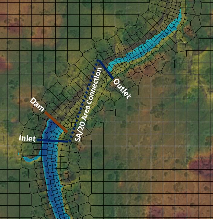
Zero-height weirs are used for cases where flow will leave a channel laterally, but there is no defined obstruction or hydraulic control separating the two.  Commonly this is used to simulate flow from a main channel up a tributary that is being modeled using a lateral structure and a storage or 2D area.  The HEC-RAS 2D manual has a table of lateral weir coefficients (Table 1). 

Table 1.  Lateral Weir Coefficients (from the HEC-RAS 2D Manual, page 3-50).

Notice the last category is “non elevated” overbank terrain.  If you wish to use the weir coefficients in this table to simulate a non-elevated weir, do not use the Zero-Height weir.  That is strictly for Hager’s equation and Hager’s method automatically computes the weir coefficient.  Instead, use the broad crested standard equation and enter in the non-elevated weir coefficient there. 

Gated Weirs. 

When modeling gated spillways at inline structures or lateral structures, users can provide a weir coefficient for flow over the spillway when the gate is completely opened, and out of contact with the flow (Figure 3). This is different from the discharge coefficient used for flow over the top of the inline structure (Figure 1). 

Figure 3. Inline Gate Editor

With gated spillways, the user has three options for the weir shape:  Broad Crested, Sharp Crested, and Ogee (Figure 4).  Broad Crested and Ogee work the same as previously discussed.  The Sharp Crested option also uses the standard weir equation but gives you three options for determining the discharge coefficient:  user-entered, compute with the Rehbock equation, or compute with the Kindsvater-Carter equation.  For both the Rehbock and Kinsvater-Carter methods, the weir coefficient will be computed independently at each time step. So you can have a varying discharge coefficient for varying heads. 

Figure 4.  Inline Gate Editor.

The Rehbock equation for the discharge coefficient was developed for rectangular weirs and is as follows:
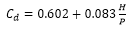
                                                                                                                 (3)
Where P = Spillway approach height.  This value must be entered to use the Rehbock equation.  HEC-RAS will then compute the weir coefficient, C using equation (2).   According to Ippen (1950), this equation holds up well for values of H/P up to 5.  And it performs with fair approximation for H/P values up to 10. 

The Kindsvater-Carter method was developed in English units only and is as follows:
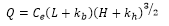
                                                                                                        (4)

Where Ce = effective weir coefficient, ft1/2/s
                kb = a correction factor to obtain effective weir crest length, ft
            kh = a correction factor with a constant value of 0.003 ft

The effective weir coefficient, Ce is a function of two ratios:  L/B and H/P, 

Where  L = Weir crest length
            B = Average width of the approach channel
            H = Energy head over the weir crest
            P = Spillway approach height

Ce is a function of both the relative width and relative depth of the approach channel and is taken from the following chart (note that the chart uses the variable h1 for H.  They are the same):

Figure 5.  Effective Weir Coefficient

kb is used to determine the effective length of the weir crest and is a function of the relative width of the approach channel.  It is taken from the following chart:

Figure 6.  Correction factor kb.

To use the Kindsvater-Carter method in HEC-RAS for a gated spillway, first select the weir shape as “Sharp Crested”.  Then select “Compute with Kinsvater-Carter eqn as the Weir Method.  You must then choose a relative approach channel width (L/b) and enter the spillway approach height, P (note, b is used in the HEC-RAS Inline Gate Editor for B.  They are the same). 

Figure 7.  Kindsvater-Carter Weir Method.

Remember, the Kindsvater-Carter equation was developed and is presented here in English units.  When using SI units, HEC-RAS will automatically convert the units appropriately.  So you can still enter a spillway approach height in meters if you are using SI units. 

The Kindsvater-Carter weir equation is built for rectangular weirs and “is particularly useful for installations where full crest contractions or full end contractions are difficult to achieve.”  (USBR 2001)  More information on the Kindsvater-Carter equation, including its limitations, can be found here:  http://www.usbr.gov/tsc/techreferences/mands/wmm/chap07_06.html

References:
Federal Highway Administration (FHWA), 1978.  Hydraulics of Bridge Waterways, Hydraulic Design Series No. 1, by Joseph N. Bradley, U.S. Department of Transportation, Second Edition, revised March 1978, Washington D.C.

Ippen, A.T. ,1950.  Channel Transitions and Controls, Chap. VIII in Hunter Rouse (editor): Engineering Hydraulics,” John Wiley & Sons, Inc., New York.  pp.496-588.

Unites State Bureau of Reclamation (USBR), 2001.  Water Measurement Manual, http://www.usbr.gov/tsc/techreferences/mands/wmm/

U.S. Army Corps of Engineers (COE), 1965.  Hydraulic Design of Spillways, EM 1110-2-1603, Plate 33.