Written by Christopher Goodell, P.E., D.WRE | WEST Consultants
Copyright © The RAS Solution 2014. All rights reserved.
Let’s say you have a digital terrain model of the area you want to model with 2D HEC-RAS. ONLY 2D RAS. In other words, you want to lay out a grid, but do not want to have do to any 1D computations-all 2D. The problem is the area you want to model includes one or more rivers and streams that have no bathymetric (under water topography) data represented in the digital terrain model. This is a common problem as many sources of terrain data are collected today using LiDAR (Light Detection And Ranging). As great as LiDAR is for collecting surface data, conventional forms of LiDAR do not penetrate water.
To adequately model 2D in RAS,

Showing posts with label Interpolation. Show all posts
Showing posts with label Interpolation. Show all posts
Monday, December 8, 2014


Monday, August 4, 2014
Exploring HEC-RAS: XS Interpolation Within a Reach-Part 2
Written by Christopher Goodell, P.E., D.WRE | WEST Consultants Copyright © The RAS Solution 2014. All rights reserved.
The last post on XS interpolation gave an overview for reasons cross section interpolation may be necessary and a detailed description of Interpolation Option A: “Within a Reach”. http://hecrasmodel.blogspot.com/2014/05/exploring-hec-ras-xs-interpolation.html
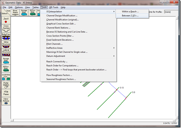
This post will cover Option B: “Between 2 XS’s”. Between 2 XS’s simply means HEC-RAS will interpolate cross sections ONLY between two selected “non-interpolated” cross sections. It will not interpolate over a reach. Obviously the disadvantage here is that you have to interpolate between pairs of cross sections one-at-a-time, which could prove to be a long exercise for a large model. However, Option B has a huge advantage over Option A, in that you are able to control how interpolation is done, by drawing your own connecting Master Chords. More on that in a bit. First, to initiate interpolation with Option B, go to the Geometric Data window and select Tools…XS Interpolation…Between 2 XS’s…
When Option B is selected, the following window will open:
The last post on XS interpolation gave an overview for reasons cross section interpolation may be necessary and a detailed description of Interpolation Option A: “Within a Reach”. http://hecrasmodel.blogspot.com/2014/05/exploring-hec-ras-xs-interpolation.html
This post will cover Option B: “Between 2 XS’s”. Between 2 XS’s simply means HEC-RAS will interpolate cross sections ONLY between two selected “non-interpolated” cross sections. It will not interpolate over a reach. Obviously the disadvantage here is that you have to interpolate between pairs of cross sections one-at-a-time, which could prove to be a long exercise for a large model. However, Option B has a huge advantage over Option A, in that you are able to control how interpolation is done, by drawing your own connecting Master Chords. More on that in a bit. First, to initiate interpolation with Option B, go to the Geometric Data window and select Tools…XS Interpolation…Between 2 XS’s…

When Option B is selected, the following window will open:
Monday, May 19, 2014
Exploring HEC-RAS: XS Interpolation Within a Reach
Written by Christopher Goodell, P.E., D.WRE | WEST Consultants
Copyright © The RAS Solution 2014. All rights reserved.
I’m starting a new series called “Exploring HEC-RAS”. Each post will discuss a feature in the menu items, starting with the Tools menu item in the Geometry Schematic. Today’s topic is “XS Interpolation Within a Reach”.

There are two options for interpolating cross sections in HEC-RAS: “Within a Reach…”, let’s call this Option A, and “Between 2 XS’s…”, Option B. First, let’s briefly review why you may need to interpolate cross sections in HEC-RAS. Cross Sections should be selected early on in your project to adequately define changes in geometry, roughness, bed slope, and discharge. Also, cross sections are needed to properly define the expansion and contraction zones around bridges, culverts, and inline structures. Additional cross sections are needed in areas of rapidly varying flow and/or significant grade breaks to avoid overestimation of energy loss (http://hecrasmodel.blogspot.com/2010/01/another-reason-for-interpolated-cross.html). There’s also that pesky warning message that seems to always pop up:

Each of these warning messages suggest that more cross sections will provide a better solution. Finally, in unsteady flow modeling, there’s a relationship between cross section spacing, wave speed, and computational time step that minimizes errors and numerical instabilities (Courant Condition). Interpolating cross sections is a quick and convenient way to satisfy this relationship.
The first interpolation method, Option A, is called Interpolation “Within a Reach…”. This is also called “blind” interpolation, because you cannot see nor control how HEC-RAS interpolates new cross sections. They are interpolated based on the internal interpolation scheme, with no user interaction, except for entering a maximum spacing value. This method is good for testing whether the spacing of cross sections will help produce a more numerically stable simulation. You can choose to interpolate over an entire river/reach, or a segment of a reach, based on your selection of the Upstream River Station and Downstream River Station.

Here you can see there’s a single input box for the Maximum Distance between XS’s. RAS will then determine the number of interpolated cross sections necessary between each set of original cross sections so that the main channel reach lengths never exceed that maximum distance. There are a couple of other options to be aware of in this window: Cut Line GIS Coordinates allows you to control whether HEC-RAS interpolates the cut line coordinates of the original cross sections, or simply displays the interpolated cross sections as perpendicular segments along the reach centerline. Whatever you select here will have no bearing on the computations, but will only change how the cross sections are displayed in the geometry schematic. If you have a georeferenced project with adequate initial spacing, the first option should display the interpolated cross sections just fine. However, if you have a very sinuous river and the original cross sections are spaced too coarsely, the interpolated cross sections may not follow the stream centerline very well, sometimes resulting in interpolated cross sections laying off center or completely away from the stream centerline (see below).


In this case, to better display the layout of the interpolated cross sections, select the “Generate for display as perpendicular segments…” option. This will lay the interpolated cross sections centered on their bank stations and perpendicular to the stream centerline.

Notice how the interpolated cross sections now follow the stream centerline. However, be aware that these new interpolated cross sections are NOT georeferenced. If you will be mapping your results on inundation maps, it would be better to cut new original cross sections around the bend section of the reach and use the “Linearly Interpolate cut lines…” option.
The dropdown box “Decimal Places in interpolated Sta/Elev” simply directs HEC-RAS to how many decimal places to carry out the station elevation points for the interpolated cross sections. The default is 2 and is generally left alone. One case where you may want more precision in the decimal places is with extremely shallow reaches, where the resulting bed profile may look “stair stepped” due to rounding off of the channel invert point. Adding more precision will help to smooth this out.
A word of warning about Interpolation Option A, “Within a Reach…”. The interpolated cross sections under this method are generated by built-in interpolation routines, that simply linearly interpolate station elevation points based on their proportional stationing within a subsection. You have no control over the interpolation. As such, it is very important that before you use these interpolated cross sections for your final RAS model, you verify that they accurately describe the geometry of the reach. If important geometric features are not captured or are improperly defined, you’ll want to get real cross sections, or interpolate using Option B, “Between 2 XS’s”. It is advised that blind interpolation (Option A) only be used to test the numerical adequacy of the cross section spacing. More on Option B in the next post. Stay tuned.
Tuesday, October 8, 2013
Stabilizing a Dynamic Unsteady HEC-RAS Model
Written by Chris Goodell
Copyright © RASModel.com. 2013. All rights reserved.
One of the most frustrating aspects of unsteady HEC-RAS modeling can be the model stabilization process. You know, you’ve gone to great lengths collecting the best survey/topo data and solid hydrology. Then you’ve painstakingly spent hours…possibly days entered all of that data only to find that once you press the “Compute” button, the model crashes. The dreaded “Red Bar”!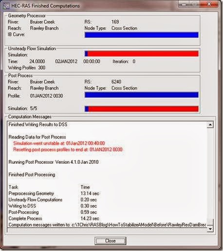 Sometimes you can get your simulation to complete without crashing, but the listed numerical errors are so high that you can’t with good conscience submit that as your final simulation. Either way, approaching an unsteady HEC-RAS model (especially a dynamic one) as a beginner with little experience and understanding of how to stabilize it can cause significant delays in your project and worse, completely blow up your budget. I’ve uploaded two HEC-RAS projects to the following Google Drive Site: https://drive.google.com/folderview?id=0B_s8OLJOgOi0YU92SGZQZm9raWM&usp=sharing
RawleyResUnstable.prj is an unsteady flow dam breach HEC-RAS project recently sent to me for help. Although the model ran to completion without crashing, it had unacceptably high errors.
RawleyResStable.prj is the fully stabilized version of the model with no numerical errors.
The following lists out the courses of action taken to stabilize the model. Feel free to download the “Unstable” and “Stable” models and try these techniques on your own. The links following some of these items will take you to more information about that particular technique.
Copyright © RASModel.com. 2013. All rights reserved.
One of the most frustrating aspects of unsteady HEC-RAS modeling can be the model stabilization process. You know, you’ve gone to great lengths collecting the best survey/topo data and solid hydrology. Then you’ve painstakingly spent hours…possibly days entered all of that data only to find that once you press the “Compute” button, the model crashes. The dreaded “Red Bar”!
 Sometimes you can get your simulation to complete without crashing, but the listed numerical errors are so high that you can’t with good conscience submit that as your final simulation. Either way, approaching an unsteady HEC-RAS model (especially a dynamic one) as a beginner with little experience and understanding of how to stabilize it can cause significant delays in your project and worse, completely blow up your budget. I’ve uploaded two HEC-RAS projects to the following Google Drive Site: https://drive.google.com/folderview?id=0B_s8OLJOgOi0YU92SGZQZm9raWM&usp=sharing
RawleyResUnstable.prj is an unsteady flow dam breach HEC-RAS project recently sent to me for help. Although the model ran to completion without crashing, it had unacceptably high errors.
RawleyResStable.prj is the fully stabilized version of the model with no numerical errors.
The following lists out the courses of action taken to stabilize the model. Feel free to download the “Unstable” and “Stable” models and try these techniques on your own. The links following some of these items will take you to more information about that particular technique.
1. Cross Section Spacing. The initial spacing was way too coarse. A visual check alone of the geometry schematic and profile plot should encourage you to investigate a finer cross section spacing.
Geometry Schematic


Profile Plot Samuels equation suggests anywhere from 15 ft to 50 ft spacing (depending on what bed slope you use). I interpolated to 50 ft for the entire reach. http://hecrasmodel.blogspot.com/2008/12/samuels-equation-for-cross-section.html


- Dam Breach models typically have time steps on the order of a minute or less. This model was initially set with a computation interval of 10 minutes which is high even for the largest and “slowest” of dam breach models. I changed the time step to 10 seconds. The selection of 10 seconds was based on “gut” feel and lots of experience doing dam breach models. There are some methods for approximating good timesteps, notably the Courant Condition and Fread’s equation. Also, setting the cross section spacing/timestep ratio equal to a representative stream velocity will get you close. In this case, the cross section spacing is 50 ft, and I was able to pull some velocities (prior to the model crashing) at about 6 ft/s. That suggests a time step of 8.3 seconds. Close enough to 10 seconds, so we’ll stick with that.
- I changed the downstream boundary normal depth slope from 0.01 to 0.001. Not sure what is downstream of the first cross section, but 0.01 is awfully steep and was setting up a very low depth at the downstream boundary (which was causing instabilities). http://hecrasmodel.blogspot.com/2010/01/downstream-boundary-normal-depth.html
Notice in the following profile plot of the downstream end of the reach how the water surface at the boundary cross section is below critical depth (the red dot). This creates an overestimation of the water depth at the next upstream cross section, which in turns creates some instability over the next several timesteps.
The proper way to handle this would be to find out what is downstream of your model and select a boundary condition that best represents those conditions. In absence of downstream conditions, the 0.001 slope for normal depth provides a reasonable solution. Either way, this underscores the importance of moving your downstream boundary far away from your area of interest in your study reach. That way the errors that do originate from your downstream boundary assumption will have diminished to negligible levels before impacting your area of interest.


- In the unsteady flow editor, the initial flow and the first time step flow should always be equal. In the original model, the initial flow is left blank (which is actually okay because RAS will use the first timestep flow if left blank). However, the first time step flow is very low at 0.14 cfs. Peak discharge of your inflow hydrograph is around 600 cfs. I put in a baseflow (minimum flow) of 5% of this, which is 30 cfs. Just to be safe, I put 30 cfs in the initial flow input box as well. It’s important to make sure that the 30 cfs baseflow does not have an impact on the peak of the breach outflow hydrograph. http://hecrasmodel.blogspot.com/2009/02/minimum-flow-requirements.html
- The upstream end of your reservoir is very steep (14%). This one was easy to spot in the profile plot because of the very nice smooth profile plot followed by a sudden spike in the energy level (green dashed line) at the upstream end. Notice to that there is a corresponding supercritical solution at the upstream most cross section. These are both indications that more cross sections are needed here. http://hecrasmodel.blogspot.com/2010/01/another-reason-for-interpolated-cross.html
I added more cross sections by interpolating the steep slope at the upstream end of the reservoir (10 ft spacing).

Notice the energy spike is not completely gone, but it is much better. Refining the HTAB parameters (http://hecrasmodel.blogspot.com/2009/02/crazy-energy-grade-line.html), turning on mixed flow and bumping up n values will collectively take care of the rest of this (see numbers 8, 9, and 10 below).

- From RS 4577 to 3791 you have your main channel defined in a small elevated side channel. The right overbank is lower in elevation than the channel.
This is problematic in RAS. Using the graphical cross section editor, I redefined the bank stations to get rid of this problem.


- Notice now in the HTAB parameters property table, the HTAB definition begins at the elevation of the invert of the side channel that was previously defined as the main channel. There is a big gap in the computation points in the newly defined main channel. This poses problems with HEC-RAS, particularly at low discharges/stages, since RAS will have to extrapolate to obtain a solution over that range.

I readjusted the cross section HTAB parameters to reflect the new bank station definitions (I used the “Copy Invert” button for all cross sections). While in there, I maximized the resolution of the HTAB parameters by changing number of points to 100 and minimizing the increment as much as possible while still having full coverage of each cross section. http://hecrasmodel.blogspot.com/2009/02/crazy-energy-grade-line.html http://hecrasmodel.blogspot.com/2011/03/more-on-htab-parameters.html

- In the figure below, notice all of the “red” areas in this zoomed in section of the upstream end of the reach.

These are areas that are near critical depth. I turned on the “Mixed Flow” option in the Unsteady Flow Analysis window, which helps stabilize the near critical depths at the upstream end of the reservoir. http://hecrasmodel.blogspot.com/2011/04/mixed-flow-regime-options-lpi-method.html If you’ve been following along correcting your own copy of the model, you’ll notice that the model now finally runs to completion without crashing. There are still a few minor errors as shown in the Computation Messages.

It’s debatable whether you need to take care of these relatively small errors. Particularly for a dam breach model, where the presumed errors of the input data probably far outweigh these small numerical errors. Nevertheless, there’s a sense of pride in putting out a very robust model, completely free of numerical errors. So…let’s continue.
- The errors in the computation window above suggest a problem around river station 6200. That happens to be the upstream end of the reservoir and the source of the error can clearly be seen with the energy grade line and critical depth turned on.

The section at the upstream end of the reservoir is very steep at about 13.5%. In fact, that’s greater than the suggested maximum slope of 10%, as stated in the HEC-RAS manuals. You can see as the pool starts to lower, the steep reach is exposed and because of the low n values, the water surface is calculated to be supercritical. Let’s assume that the geometry is correct, and the upstream end of the reservoir really is that steep. Jarrett’s Equation suggests very high n values should be used here (~0.2), based on the bed slope and hydraulic radius (after the breach when the reservoir has drained). The original model had 0.07 and 0.035 for the overbanks and main channel, respectively. I changed all the n values in this steep reach to 0.15, because I think 0.2 might be a little overkill. http://hecrasmodel.blogspot.com/2009/12/n-values-in-steep-streams.html
There…no errors! However, there is still a Warning about extrapolating above/beyond the rating curve at a bridge (R.S. 277).

- To get rid of that warning, I increased the HTAB headwater maximum elevation at River Station 277 (the bridge) from 278 ft to 280 ft so that RAS doesn’t have to extrapolate.

There we have it. A clean solution. No errors, no warnings.

Tuesday, January 19, 2010
Another Reason for Interpolated Cross Sections
Written by Chris Goodell, P.E., D. WRE | WEST Consultants
Copyright © RASModel.com. 2010. All rights reserved.
Here’s a classic case for interpolation of cross sections in a RAS model.

Notice the drop in water surface to near critical depth at the grade break. Then, at the next cross section upstream of the break, RAS seems to overestimate the head loss. Sometimes this phenomenon can be much more dramatic, occasionally initiating oscillations upstream of the break that can lead to instabilities.
When scanning the results of your model run, or when trying to diagnose sources of instability, keep an eye out for this phenomenon. Interpolation of cross sections around this point will provide a much more accurate and stable answer. Notice in the figure below, that further interpolation upstream of the newly interpolated reach is probably warranted.

Copyright © RASModel.com. 2010. All rights reserved.
Here’s a classic case for interpolation of cross sections in a RAS model.

Notice the drop in water surface to near critical depth at the grade break. Then, at the next cross section upstream of the break, RAS seems to overestimate the head loss. Sometimes this phenomenon can be much more dramatic, occasionally initiating oscillations upstream of the break that can lead to instabilities.
When scanning the results of your model run, or when trying to diagnose sources of instability, keep an eye out for this phenomenon. Interpolation of cross sections around this point will provide a much more accurate and stable answer. Notice in the figure below, that further interpolation upstream of the newly interpolated reach is probably warranted.

Subscribe to:
Posts (Atom)