Getting Profile Output in a 2D Area

Written by Christopher Goodell, P.E., D.WRE  |  WEST Consultants 
Copyright © The RAS Solution 2016.  All rights reserved. 

Back in September 2015, I wrote an article on how to extractflow data from a transect in a 2D area.   This was a round-about way of getting flow flux data out of RAS Mapper.  Back then the beta version of HEC-RAS 5.0 was somewhat limited in the ways data could be extracted from a 2D area.  In the final release of Version5.0, you may have noticed in the bottom left-hand corner of RASMapper, there is a very unassuming tab called “Profiles Lines”. 

Profile Lines are another way of extracting linear data from a 2D area, only these are extracted longitudinally, like a profile plot.  Here’s how it works:

Tuesday Tip of the Week–Axis Zooming for True Peak Discharge

Written by Christopher Goodell, P.E., D.WRE  |  WEST Consultants

Copyright © The RAS Solution 2014.  All rights reserved.

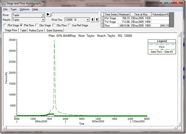
Another simple, yet very convenient tool not found discussed in the manuals is the ability to zoom in on one of the axes of a graphical plot.  This is especially useful when trying to determine if you’ve captured the true peak discharge in a steeply rising hydrograph.  Take the following example: an unsteady flow dam breach output flow hydrograph.

Here we have a steeply rising flow hydrograph from a breach at the inline structure that appears to have a peak discharge of about 35,000 cfs.  To visually inspect whether or not this hydrograph captures the true peak, we can zoom in on the x axis by clicking and dragging a “bar” on the axis itself.  Simply place your cursor just below the x axis line, on the axis labels (in this plot, the time, in hours), then click and drag a red bar bracketing the portion of the hydrograph you wish to zoom in to.

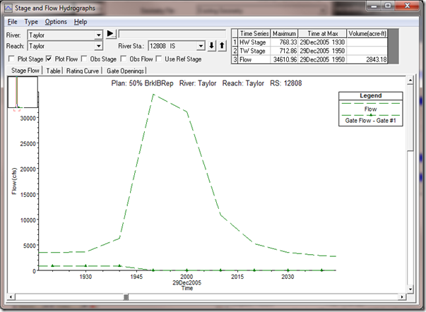
Once you release the mouse button, the plot zooms in only on the x axis, in effect “spreading” out the hydrograph so that the peak is more apparent.  Notice that the full range of discharges still appear in the plot, we’ve simply truncated the time window to a more visually convenient range. 

Now notice we can see that because the hydrograph output interval is set too coarse (in this case every 10 minutes), we miss out on the true peak of the discharge hydrograph.  It happens somewhere between 1950 hours and 2000 hours.  By rerunning the model with a smaller hydrograph output interval, we can capture a better representation of the true peak discharge.  In the next figure, the discharge hydrograph is shown for the same location with a 2 minute hydrograph output interval.

After zooming in again on the x axis, we can see that we have a much better representation of the true peak of the discharge hydrograph, which is closer to 42,000 cfs, versus the 35,000 cfs shown in the first simulation:

The axis zooming feature works on any plot (input or output) and you can zoom on either the x or y axis.  So next time you’re evaluating hydrographs, or simply wish to have a better view of a curve in any of the plots, give the axis zooming feature a try.

Negative Flows over Inline and Lateral Structures

Written by Chris Goodell | WEST Consultants.
Copyright © RASModel.com. 2013.  All rights reserved.

Though it’s not very common, it is possible to get negative flows over inline structures for unsteady flow simulations.  It’s much more likely you’ll see negative flows over a lateral structure though.  Negative flows are simply discharges in your model going the opposite direction than what you have defined as the downstream direction (or primary flow direction).  This can occur in tidal areas, backwater, or complex looped networks.  For lateral structures, you may have water spill out of your river over a lateral structure and into a storage area.  Once the flood wave passes, the head level in the storage area is higher than the river and water flows back into the river (negative flow).  It’s called negative flow because RAS will show it in tables and plots as a negative number. 
Recently, an HEC-RAS output table issue was brought to my attention, directly related to negative flows over weirs. 
“I was looking through the HEC-RAS file for the XYZ model for the 72-hr PMF and came across the following.  Do you know what -1.#INF means?”

In this example, the water surface elevation downstream of the inline structure exceeds the water surface elevation upstream of the inline structure between the time of 1420 hrs and 1900 hrs on 02 January, 1913.  During this time range, we have a negative head differential and thus a negative flow over the inline structure (from downstream to upstream).  During a simulation, when an inline structure is overtopped by water, RAS uses the same equation (the weir equation with adjustments for submergence) regardless of the direction of flow over the inline structure.  The -1.#INF is the double precision floating point default return in the Visual Basic programming language for any unreal number (i.e. you may remember imaginary numbers, “i” from high school math class).  Well RAS is trying to take a negative number (in this case the head differential) to a non–integer power, (1.5 for the weir equation, Q = CLH^1.5).  There is no real solution for this.  The good news is, this is only happening in the table, as RAS recomputes the Q Weir to populate the table using the steady flow engine.  Presumably, that is why RAS cannot deal with negative head differentials, since there is no negative flow in steady flow modeling.  During the unsteady flow computations, RAS correctly removes the negative sign to do the computations and then replaces it to show flow in the “negative” direction.  That’s why the computations work and why the Q Total is negative (which is presumably what Q Weir should be in this example).  So, in short, the unsteady flow computations are fine-the solution is correct.  The problem comes when reporting results to the Inline Structure Table.  Hopefully this will be fixed for the next version of HEC-RAS.  Until then, you can use the stage and flow output hydrographs to verify the total and weir Q’s. 

HEC-RAS File Types

Written by Aaron A. Lee 
Copyright © RASModel.com. 2013.  All rights reserved.

Behind the scenes, HEC-RAS automatically creates a series of input and output files when working with a model. It is important to know what each of these files does and how they fit into the overall scheme of your project. Keeping track of these files in an organized manner is good practice, especially as your models grow in size and complexity. This post will feature a steady flow example project, and will list common HEC-RAS files that you’ll see for Unsteady flow, Sediment Analysis, Water Quality, and Hydraulic Design projects.  Although these examples all use the number "01" in the extension, RAS can have multiple instances of each of these files for a given project (except the .prj-only one of those).  Numbers can go as high as "99" and are assigned in the order in which the files were created.   This screenshot is a folder containing the input files generated by RAS after opening and saving one of the installed example projects. At the very least, you need these input files to run the model. If someone asks you to send them your model, these files must be sent, at a minimum. Differences between Steady and Unsteady files are listed when relevant.

• .prj is the Project file. Contains current plan files, units and project description.
• .g01 is the Geometry file. Cross-sectional data, hydraulic structures and modeling approach data are stored here.
• .f01 is the Steady Flow file. Profile information, flow data and boundary conditions written in this file.
• For Unsteady Flow, .u01 is the flow file extension. This is where hydrographs and initial conditions are stored, as well as any user-defined flow options.
• For Quasi-Unsteady Flow (for a sediment analysis), .q01 is the flow file extension.
• .p01 is the Plan file. Contains a list of the associated input files, and all simulation options.

These are all text files and can be directly read and edited in a text editor. The following screenshot shows the input and output files after the steady flow model has been run. Note that some of these are only used by RAS as intermediate files during computations.

• .O01 is the Output file. Contains all of the computed results from the associated plan. This file is written in binary format and can only be read from the user interface.
• For Unsteady Flow, a .dss file is automatically generated as an output. This file contains time series data that is viewable by any program that can read dss files (typically HEC software).
• If your model links to a dss file for use as input data (e.g. inflow hydrographs, stage hydrographs, observed data, etc.), then that .dss file will be necessary to run the model and should be included in your group of files you send to a reviewer.
• .r01 is the Run file for steady flow analysis. Contains all of the necessary input data required for the RAS computational engine. The run file is created during the model simulation, and is not required to view final results.
• For Unsteady Flow, .x01 is the extension.
• .comp_msgs.txt is the Computational Message text file. Records the computational messages that pop up in the computation window. The messages file is not required to view final results, but can be useful in troubleshooting errors identified by RAS.
• .hyd01 is the Detailed Computational Level output file. This can be switched on in the Unsteady Flow Analysis window.
• .p01.rst is a Restart File (also called a Hot Start File, or Initial Conditions File). This option can be switched on by the user in the Output Control Options window. See the Hot Start post for more guidance.

For Unsteady Flow analysis, these files are categorized as “intermediate,” which means that they are not essential for running a model or viewing results, since they are recreated by RAS during run-time.

• .c01 is the Geometric Pre-Processor output file. Contains the hydraulic properties tables, rating curves, and family of rating curves for each cross-section, bridge, culvert, storage area, inline and lateral structure. This file is rewritten each time you change your geometry file.
• .b01 is the Boundary Condition file.
• .bco01 is the Unsteady Flow Log output file.
• .p01.blf is the Binary Log file.
• .IC.O01 is the Initial Conditions file.

If submitting your final model to a client or a reviewer, you will likely only send the necessary input files. Sending output files are optional, but will allow the reviewer to avoid rerunning the model on their end. Including the .c## files might be a good idea for larger models so that RAS can skip the pre-processing step. SEDIMENT ANALYSIS

• .S01 is the file extension for Sediment Data. This file contains flow data, boundary conditions, and sediment data.
• .SedCap01 is the extension for Sediment Transport Capacity data. When sediment transport computations are performed, RAS creates a set of intermediate files:
• .sed is the detailed sediment output file.
• .SedHeadXS01 is the header file for the cross section output.
• .SedXS01 is the cross section output file.
• .H01 is the Hydraulic Design data file.
• .H01.SiamInput is the SIAM Input Data file.
• .H01.SiamOutput is the SIAM Output Data file.

WATER QUALITY ANALYSIS

• .W01 is the file extension for Water Quality data. This file contains temperature boundary conditions, initial conditions, advection dispersion parameters and meteorological data. When water quality computations are performed, RAS creates a set of intermediate files;
• .bco is the water quality log file.
• .p01.wqrst01 is the water quality restart file.
• .color_scales is the file that contains the water quality color scale.

Remember that file extensions can be numbered from 01 to 99, and are assigned in the order that they are created.