Written by Aaron A. Lee | WEST Consultants
Copyright © RASModel.com. 2011. All rights reserved.
By using the Mixed Flow Regime option for Unsteady Flow Analysis, RAS can better handle transitions from subcritical to supercritical flow. This option should be utilized only after determining that a mixed flow situation exists, which requires judgment from the modeler. One application where this could be particularly useful is dam breach modeling, or any other extreme and flashy flood event. Even though a model is stable there may still be small errors in the solution (caused by max. iterations). The Local Partial Inertia (LPI) factor may eliminate or reduce these errors, particularly if they occur when the Froude number is near 1. Figure 1 shows the Unsteady Flow Analysis window with the Mixed Flow Regime option selected. This post will focus on the LPI Filter, which is enabled when Mixed Flow Regime is selected by the modeler.
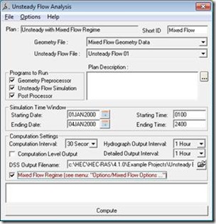
Figure 1. Unsteady Flow Analysis Window
Once the Mixed Flow Regime option is selected, additional settings can be adjusted to help stabilize the model. Navigate to
Options, Mixed Flow Options. This window, shown in Figure 2, allows the user to adjust two inputs for the LPI factor.
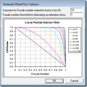
Figure 2. Mixed Flow Options Window
For the unsteady flow computation scheme, RAS accounts for a local acceleration and convective acceleration (inertial terms) through the St. Venant equation of Conservation of Momentum. The St. Venant equations, and by extension, HEC-RAS, are designed to work best in gradually varied flow. Transitions from supercritical to subcritical flow (hydraulic jump), and to a lesser extent subcritical flow to supercritical flow, are rapidly varied flow situations. These are not gradual changes, in the hydraulic sense. Near critical depth (Froude number approaching 1) the convective acceleration terms can change very rapidly over a short distance (think of a hydraulic jump) and can lead to oscillations in the solution. These oscillations tend to grow larger until the solution goes completely unstable (HEC, 2010). The LPI factor systematically reduces these inertial terms to dampen the oscillations, helping to stabilize the model. The user can influence the magnitude of reduction by varying the two inputs in Figure 2.
The first input, m, is the exponent for Froude number reduction factor. Its default value is 10 and ranges from 1 to 128. Adjusting m will change the shape of the curve on Figure 2, thus influencing the rate of reduction of the inertial terms. You can see that by making m smaller there is an earlier and more direct reduction in the inertial terms, with respect to the Froude number. Increasing m can make the model more accurate but increases the likelihood of numerical instability.
The second input, F
T, is the Froude number threshold at which the LPI factor is set to zero. In other words, if the calculated Froude number at the current cross-section is larger than F
T the inertial terms will be eliminated from the computations at that cross-section for the current computational time step. The default value is 1. Making F
T smaller will improve the stability of the model, but will also reduce the accuracy. A larger F
T can make the model more accurate, but increases the likelihood of numerical instability as the inertial terms will be more sensitive to fluctuations in Froude number.
A good place to start is to run the simulation with the default values
Technorati Tags:
HEC-RAS,
RAS,
Mixed Flow,
LPI Method,
Unsteady Flow,
Supercritical,
Subcritical,
Hydraulic Jump,
Froude,
Water Surface Profile,
Dam Breach,
Dam Break,
Flood,
Numerical Model,
St. Venant
and see what the profile looks like. For this flume example, the model ran without reporting any maximum water surface errors. The profile for the default LPI inputs is shown in Figure 3.
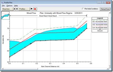
Figure 3. Profile Plot, Default Values
Next, a value of 1.6 was chosen for F
T. This simulation yielded small maximum water surface errors, but had maximum iterations at various locations. The value of m was left unchanged. Figure 4 shows the results.
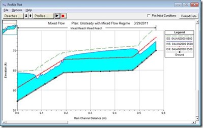
Figure 4. Profile Plot, Increased Froude Number Elimination Threshold
Even though the errors were small, instabilities could be seen in the downstream end. Notice the instabilities around the transitions between the flow regimes. The value of m was reduced from the default of 10 to 7 in order to improve the stability of the model. Figure 5 shows the profile for reduced m and increased F
T. The modeler should choose the largest values of m and F
T that produce a stable model. However, check the results to make sure that the output is reasonable. Notice how the transitions between flow regimes are much better defined in Figure 5 then the default setup shown in Figure 3. That’s because the default LPI parameters (m = 10 and F
T = 1) provide dampening of the results. Though Figure 3 looks very stable (and it is), Figure 5 (m = 7 and F
T = 1.6) is both stable and (by my engineering judgment) more accurate. Also, notice how the slight increase in energy (green dashed line) is less in Figure 5 versus Figure 3. An increase in the energy elevation in the direction of flow is an indication of error in most cases. Further adjustment of the LPI parameters may help to eliminate the error in the energy grade line, while still producing a stable solution.
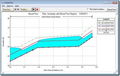
Figure 5. Profile Plot, Increased Froude Number Elimination Threshold and Decreased Exponent ,m


