Preview of the new Finite-Volume Approach for 1D Reaches

One of the most anticipated new features soon to come in the next major version of HEC-RAS (Version 5.1) is the option of running unsteady 1D reaches with a finite volume solution scheme.  This will be a fantastic addition to HEC-RAS.  Gary Brunner recently gave me a brief overview of the new finite volume feature we can expect.  But before you ask, there is no set release date for Version 5.1 yet.  But I'm hoping we'll see it within the next year or two.

1D Finite Volume Solution Algorithm

By Gary W. Brunner, P.E., D.WRE

Senior Technical Hydraulic Engineer

Hydrologic Engineering Center

A brand new solution algorithm has been developed for 1D modeling.  A Finite-Volume solution approach, similar to what was added for 2D modeling will be available for 1D modeling in HEC-RAS version 5.1.

The current 1D Finite Difference solution scheme has the following deficiencies:

1. Cannot handle starting or going dry in a cross section
2. Low flow model stability issues with irregular cross section data
3. Extremely rapidly rising hydrographs can be difficult to get stable
4. Mixed flow regime (i.e. flow transitions) approach is approximate
5. Stream junctions do not transfer momentum

The new 1D Finite Volume approach has the following positive attributes:

1. Can start with cross sections completely dry, or they can go dry during a simulation (wetting/drying)
2. Very stable for low flow modeling
3. Can handle extremely rapidly rising hydrographs without going unstable
4. Handles subcritical to supercritical flow, and hydraulic jumps better.
5. Junction analysis is performed as a single 2D cell when connecting 1D reaches (continuity and momentum is conserved through the junction).

Additionally, the new 1D Finite Volume approached is solved in the same matrix as the 2D equations.  Solving in the same matrix allows for faster 1D/2D model solutions and more accurate flow transfers between 1D and 2D elements.  The equations are solved together and all hydraulic connections are updated together on an iteration by iteration approach, rather than separately, as in previous versions of HEC-RAS.

Using a HEC-RAS Storage Area and Lateral Structures to Replace Standard Reach Junctions

Written by Lonnie Anderson, P.E., CFM  |  Pape-Dawson Engineers, Inc.
Copyright © The RAS Solution 2018.  All rights reserved.

Situation:

Advances in HEC-RAS now allow for improved simulation of overbanks using 2D Flow Areas. Coupled 1D/2D models where 1D cross-sections represent the bank-to-bank cross-section data and 2D flow areas represent overbank areas has greatly improved the accuracy and robustness of HEC-RAS models. This is particularly the case in flat, urban areas with significant overbank flow paths.

These coupled 1D/2D models have highlighted several simplifications and shortcomings of the traditional HEC-RAS Junction methodology. Note that the standard method is still required in 1D steady flow modeling.  The following points suggest an alternative Junction method is worth considering when building a coupled 1D/2D model.

 Figure 1 - Traditional HEC-RAS Junction Methodology with a Coupled 1D/2D Unsteady Model - Simple Junction

• 1D to 2D offline flow transfer over the junction length is not possible in HEC-RAS.  In other words, a lateral structure cannot span across a junction. In complex confluences, this transfer region may be critical. Simply reducing the distance between bounding cross-sections to minimize this region may not be an option depending on the channel and bank alignments (see Figure 1). 

• The volume of water within the bounding cross-sections of junctions is not accounted for, whether forcing the water surface elevation to match the downstream bounding cross-section or using the Standard Step one dimensional Energy equation. Both solution techniques simplify the hydraulics of the region, and in particular, the main reach which conveys the greatest volume (see Figure 1).

Simplification of Junction hydraulics has been “accepted” as reasonable, as                          demonstrated by the following guidance from the USACE-HEC: 

Combining Two Reaches or Splitting One

Written by Christopher Goodell, P.E., D.WRE
Copyright © The RAS Solution 2015.  All rights reserved.

Suppose you have two separate HEC-RAS rivers and wish to combine them.  There is no “combine two rivers” option in HEC-RAS, but it can be done using the Move Points/Objects option.  Take the very simple reach presented below:



I wish to combine the Upper Tualatin with the Clackamas reach of the Willamette River.  In the figure above, they are disconnected-two separate rivers.  Select Edit…Move Points/Objects and

Modeling Junctions for Unsteady Flow Analysis

Written by Aaron A. Lee   | WEST Consultants
Copyright © RASModel.com. 2011. All rights reserved.

In the current version of HEC-RAS (v 4.1.0) there are two methods of modeling the hydraulics at a junction for unsteady flow. By default RAS selects the Force Equal WS Elevations (Forced) method, which forces the upstream bounding cross-sections’ water surface equal to the downstream water surface. This method may be adequate for some situations like high depths and shallow bed slopes, but can also cause major instabilities in your model if depths are too low and/or bed slopes are too steep. The alternative is the Energy Balance (Energy) method, which uses the energy equation across the junction to solve for WS elevations. The model presented in this post is part of a dam breach simulation and will demonstrate that there can be significant differences between the two methods. This simulation is a hotstart run which seeks to identify stability issues by starting the downstream stage artificially high, and slowly lowering it to the true solution over the run time. The river system in this model has a normal flow combining junction with a steep transition. Special attention will be paid to the steep transition, especially at low flow conditions. The Figure 1 below shows the 3D view of the model extents, which includes the Middle Reach, Tributary C and Lower Reach.


Figure 1


For a normal flow-combining junction, the water surface elevations at the upstream bounding cross-sections are based on the computed downstream WS elevation. Longer lengths between the bounding cross-sections will generally make your results less accurate and less stable. By looking closely at the above figure you can see that the bounding cross-sections are spaced far apart, which corresponds to long junction lengths. The results for both methods are shown below in a series of profile plots. Figures 2a and 2b show the junction approximately halfway through the simulation. Figure 2a shows the Energy Balance method and Figure 2b shows the Forced Equal Water Surface method. The water surface is high enough that there are no differences between the two methods. For reference, Tributary C is the steeper of the upstream reaches.


Figure 2a


Figure 2b


Significant differences develop in Figures 3a and 3b as the downstream stage is lowered. At the same time-step, the two profiles are dramatically different. The Forced method produces a large drop at the junction (Figure 3b), while the Energy method produces only a minor instability (Figure 3a). The large drop (shown in Fig. 3b) occurs because RAS must balance the momentum equation from the upstream bounding cross-section at the junction (an unrealistically low water surface) to the cross-section immediately upstream. The only way to provide a balance is to overestimate the upstream WS elevation, which is why the profile for 3b is much higher than 3a. Notice the spike in the energy grade line. The same problem occurs for the Energy method, but at a much smaller degree.


Figure 3a

Figure 3b


Figures 4a and 4b show Tributary C only, just prior to the model crashing for the Forced Equal Water Surface method. There are obvious oscillations in the profile plot, which indicates a very unstable solution. As the stage is lowered downstream, the WS elevation at the junction also becomes lower. At a certain point the WS elevation at the junction approaches the invert for the upstream cross-section; and the model crashes. Figure 4b shows a zoomed in view of the WS elevation relative to the invert of the channel as the channel runs dry.

Figure 4a

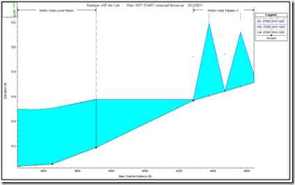
Figure 4b


The best solution is to shorten the junction lengths as much as possible, which is done by adding cross-sections closer to the junction. By adding additional cross-sections you are decreasing the length over which RAS makes its calculations, which helps to remove the problems with low water surface elevations over a junction. If surveyed data is unavailable, then start by copying the most downstream cross-sections of the upstream reaches to a location closer to the junction. The positioning of these new cross-sections will be based on the judgment of the modeler, who should know the actual conditions of the river system. Make sure to adjust the downstream reach lengths and junction lengths accordingly.


In this example, cross-sections were placed within 20 ft of the junction. Junction lengths were changed from 573’ and 534’ to 35’ and 28’ for Tributary C and Middle Reach, respectively. In addition, cross-sections were added every 40’ on the steep section of Tributary C by interpolation. Figures 5a and 5b each show the profile plots for both the Energy and Forced method at the junction of Tributary C and Lower Reach.

Figure 5a

Figure 5b


By redefining the geometry around the junction the error is significantly reduced for both methods and the results appear stable. Both profiles are very similar in this case, showing only a slight difference in WS elevations. The dotted line-type represents the profile for the Forced method. It might not always be possible, or realistic, to place new cross-sections close to the junction. The Energy method allows this model to run to completion without the addition of new cross-sections, though the results appear to not be as good. The table below lists the WS elevations at the bounding cross-sections for each of the different plans: the initial Energy method, and the Forced and Energy method after adding additional cross-sections.













The initial plan has the geometry with the long junction lengths, which consistently calculates lower WS elevations than the plans with shorter junction lengths. Although the elevations were underestimated in the initial runs, they are still within 1 ft of the new profiles. For this model, the Energy method provides a stable solution at the junction without having to modify the geometry. However, given the steepness of Tributary C, the addition of cross-sections near the junction improved the accuracy and stability of the model output. Therefore, even though the Energy method can produce stable results for long junctions in steep reaches, adding more cross sections will improve the results.