How to draw cross sections.

Written by Chris Goodell, P.E., D. WRE
Copyright © RASModel.com. 2012. All rights reserved.

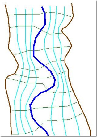
Cross sections must be perpendicular to the flow lines at all locations.  And they cannot intersect with each other.  That is why it is common to see cross sections snap at different angles outside the main channel (we call this doglegging).  The trick is to keep them from intersecting, while also staying perpendicular to flow lines.  In the figure below, the dark blue line represents the main channel.  The brown lines represent the edge of the flood plain.  The light blue lines are my impression of the flow lines through this terrain, if water were flowing appreciably in the floodplain.  The green lines are cross sections.  Notice that the cross sections are drawn so that they are not only perpendicular to the main channel, but also to my perception of the flow lines in the floodplain.  It can be very helpful to draw these flow lines before cutting cross sections. 

It takes a little bit of practice to do this correctly, and most of the time some trial and error, but as long as you remain perpendicular to the flow lines and don’t intersect, you’ll have a good set of cross sections. 
Where it can get tricky is at a junction.  The following RAS Bloggery article will help with junctions.  http://hecrasmodel.blogspot.com/2009/02/how-to-best-model-junction.html

Q & A: Flow Attenuation

Written by Chris Goodell, P.E., D. WRE | WEST Consultants
Copyright © RASModel.com. 2012. All rights reserved.

Question: 
When running an unsteady flow model with a single inflow hydrograph, why does my discharge decrease in the downstream direction for a given output profile? 

Answer: 
This is called flow attenuation.  You see this to varying degrees in all unsteady flow models and it is a real phenomenon.  The shallower the reach, or the wider the floodplain, the more pronounced this effect will be.  In very steep streams, you may not notice flow attenuation at all. 
The physical process is as follows:  As the flood level rises, water moving downstream fills in available volume.  This volume is called storage.  Water going into storage is taken away from the flow going downstream and that is why you see a decrease in discharge as you move in the downstream direction.  Wider floodplains and shallower reaches have more available storage volume, which is why flow attenuation is pronounced under these situations.  Once the flood wave passes, and you are on the receding limb of the flood hydrograph, the water that had gone into storage now returns to the active discharge.  In this case you’ll see an increase in flow as you move in the downstream direction.  Notice in the figure below that the discharge at time 0042 (before the peak of the flood wave) decreases in the downstream direction, while the flow at time 0124 (after the peak of the flood wave) increases in the downstream direction.

You can also see this effect when viewing hydrographs in the figure below from two cross sections, one upstream (River Station 2500) and one downstream (River Station 2400).  The attenuation of flow is the difference in peak discharge between these two hydrographs-in this case, about 2.3 cms.  The area between these two curves represents a volume of water.  The area to the left, where the upstream discharge is greater than that downstream discharge, represents water going into storage.  The area to the right, where the upstream discharge is less than the downstream discharge, represents water leaving storage.

Attenuation is included in the conservation of mass equation, which is one of the two equations (the St. Venant equations) used to define the movement of water through a reach in HEC-RAS-the other being conservation of momentum.    From the HEC-RAS Hydraulic Reference Manual (Page 2-22), “Conservation of mass for a control volume states that the net rate of flow into the volume be equal to the rate of change of storage inside the volume.”    In other words, Inflow minus outflow equals the change in storage over time.  The equation is:

where A = flow area, Q equals discharge, t = time, and x = length. 
The discretized form of this is more practical to use and may be more familiar: 

Where I = Inflow to a discrete control volume, O = Outflow, DS = Change in Storage, Dt = time duration (i.e. time step).

Coefficients of Contraction/Expansion at Bridges.

Written by Chris Goodell, P.E., D. WRE | WEST Consultants
Copyright © RASModel.com. 2012. All rights reserved.
In HEC-RAS, it is a well known modeling technique to increase the coefficients of contraction and expansion in the vicinity of a bridge for steady flow modeling. 
This is done to capture the energy loss resulting from increased flow contraction approaching the bridge, and increased flow expansion when leaving the bridge.  This energy loss is not accounted for in the friction loss, so HEC has added in the ability to account for it using the contraction and expansion coefficients, multiplied by the difference in velocity head between two cross sections.  Typically, RAS modelers will apply the higher coefficients (0.3 for contraction, 0.5 for expansion) at Cross Sections 4, 3, and 2 of the traditional cross section layout for bridges (see figure at the bottom of this post).  Cross Section number 1 (the most downstream of the 4-cross section layout) is typically left at the default values of 0.1 and 0.3, respectively.  A common question is “why is Cross Section #1 left with the default values?”
The coefficients of contraction and expansion are applied to the reach from the cross section at which they are defined to the next cross section downstream.  In the energy equation,
, h_e represents the head loss from one cross section to the next.  The equation for head loss, h_e, is:

Where C is the coefficient of contraction or expansion.  Subscripts 1 and 2 represent the two neighboring cross sections.  So here you can see clearly that the coefficient of contraction or expansion is applied over a reach, defined by L, which is the length between Cross Sections 1 and 2.
So, for bridge modeling, the reach from Cross Section 4 to 3 defines the zone of contraction as flow approaches the bridge.  The higher coefficients are applied to Cross Section 4 in this case.
The reach from Cross Section 3 to 2 defines the fully contracted zone though the bridge.  You could make a case that since the flow is fully contracted in this zone, that the typical coefficients should be used (0.1 and 0.3).  However, since there is usually a higher amount of turbulence in this zone, traditionally everyone keeps the higher coefficients (0.3 and 0.5).  The higher coefficients are applied to Cross Section 3 in this case.
The reach from Cross Section 2 to 1 defines the expansion zone downstream of the bride.  The higher coefficients are applied to cross section 2 in this case.
At Cross Section 1 and further on downstream, the flow is considered fully expanded, so Cross Section 1 maintains the typical coefficients (0.1 and 0.3). 

How to get a table of Peak Flows and Peak Stages for Unsteady Simulations

Written by Chris Goodell, P.E., D. WRE | WEST Consultants
Copyright © RASModel.com. 2012. All rights reserved.
This is a common question.  It’s often desirable to have a table of timing for peak stages and flows for dam breach models.  This allows you to track the arrival of the flood wave at all locations downstream of the dam.  However, the typical output plots in HEC-RAS are not very helpful in providing this information.  You could look at each cross section’s stage and flow hydrograph, and pick off the time for the peaks, but this can be very tedious and time-consuming.  There is a much faster way to get this information using the DSS Viewer in HEC-RAS.

Go to the DSS viewer on the main RAS window.

Once there, filter the records as follows by clicking in the blank cell at the top of each column and selecting what you want to see from the dropdown box:

Part A: Select the Reach you want to look at
Part B: Leave Blank
Part C: Select LOCATION-TIME
Part D: Leave Blank
Part E: Select MAX STAGE or MAX FLOW
Part F: Select the Plan you want to view.


Once you have the record you’re interested in, double click it in the filter table so that it is brought down to the list box at the bottom. Then highlight the record in the list box and click “Plot/Tabulate Selected Pathname(s). You should see a graph that plots out the Simulation Time for Max Flow or Stage for every cross section in the selected reach.

For peak stage…



For peak flow…



Within the DSS Plot window, select the “Table” tab to see tabular output.

Permanent and Non-Permanent Ineffective Flow Areas

Written by Chris Goodell, P.E., D. WRE | WEST Consultants
Copyright © RASModel.com. 2011. All rights reserved.
The traditional way of changing non-permanent ineffective flow areas to permanent involves going through each cross section, one at a time, in the cross section editor, selecting Options…Ineffective Flow Areas, and then manually checking which ineffective flow areas to make permanent. 

This can be long and tedious if you have a lot of cross sections to change.  HEC-RAS has an easy-to-use method for changing ineffective flow areas from non-permanent to permanent for multiple cross sections.  In the geometry editor, select Tools…Ineffective Areas…Set to Permanent Mode.  

Here you select the cross sections with which you want to change the non-permanent ineffective flow areas to permanent, and RAS will do that for you.  If you have a lot of cross sections where you want to do this, this utility is much faster than the traditional way of selecting each individual cross section in the cross section editor and manually changing the status.

There are a couple of disadvantages to the former method:  First, with the traditional method, if you select a cross section to have its ineffective flow areas changed to non-permanent, all of the ineffective flow areas will be changed for that cross section.  You cannot pick and choose within one cross section.  Second, once you have changed a cross section’s ineffective flow areas to permanent, there is not a similar multiple cross section selection utility to go back to non-permanent. 

Dr. Ray Walton, of WEST Consultants passed along a very easy way around this second disadvantage.  First, open up the geometry file (*.g##) that you want to edit in a text editor.  Wordpad, Notepad, WORD will all do.  Go to the search tool and search on the string “       T”.  That’s 7 spaces followed by a “T” which means “true”.  This string is used in the text editor to indicate an ineffective flow area is permanent.  Simply replace that text with “       F” (seven spaces followed by an “F”). 



A simple “search and replace” action will allow you to make this change for a number of cross sections very quickly.  If you have specific cross sections you wish to do this to, first search on the River Station.  In the example above, the River Station is “11576”.  Then scroll down to “       T” and change it to “       F”. 

As always, be very careful when editing a RAS file directly in a text editor.  It's very easy to corrupt the file if you make a small mis-type (i.e. you put in 6 spaces instead of 7 before the "F").  I always suggest making a copy of the original file for safe-keeping, before you make your edits. 

Theta Implicit Weighting Factor and its Effect on Sample Datasets

Written by Aaron A. Lee   | WEST Consultants
Copyright © RASModel.com. 2011. All rights reserved.
Adding to the previous topic on the Theta Implicit Weighting Factor (Theta), this post takes an objective look at how the unsteady-flow option affects model output. Theta is a weighting factor for the spatial derivative used in solving the finite difference forms of the St. Venant equations. Adjusting Theta can improve model stability or increase the accuracy of the output. In a practical sense, how much is Theta really changing the solution? This post observes the influence of Theta by running the 21 installed (sample) projects in HEC-RAS version 4.1.

Theta can be found by navigating to Calculation Options and Tolerances under the Unsteady Flow Analysis Options menu. The default value is 1.0, but the user can define a value of Theta anywhere between 1.0 and 0.6. A value of 0.5 represents a half weighting explicit to the previous time step’s known solution, and a half weighting implicit to the current time step’s unknown. A value of 1.0 gives a fully implicit formula that is highly diffusive. In theory, a higher value will improve model stability but is less accurate in the solution. The opposite is true for lower values of Theta, which can make the model more sensitive to errors and lead to oscillations.

The table below summarizes the results for the sample projects included in the experiment. Water surface elevations (WSEL) are compared at each river station between the current plan and the default plan, Theta = 1.0. The values in the table are the largest maximum differences in WSEL for the entire reach. The cells in red are the plans that failed.



Apart from the three crashed runs, the difference in the solutions is very small. The results demonstrate that for these simulations, the model is not highly sensitive to changes in Theta. Keep in mind that these models are relatively simple (shorter reach lengths, plain structures, uniform geometry) when compared to other unique project situations.

Changing Theta has a direct effect on how the solution is solved, but other factors may have more of an effect on stability and accuracy. The Hydraulic Reference Manual notes that factors such as cross-sectional properties, abrupt slope changes, flood wave characteristics, and complex hydraulic structures often overwhelm any stability considerations associated with Theta. When testing a model, pay special attention to the stability considerations listed above before laboring over Theta. While lowering Theta will yield (technically) more accurate results, it can also propagate errors where other factors may be causing problems. The User’s Manual suggests making sure that the computation interval is accurately defined, and that the maximum number of iterations is reasonable.

The HEC-RAS User’s Manual (page 8-32) suggests starting out with a Theta value of 1.0. Paraphrasing from the User’s Manual, page 8-32: “Once the model is up and running, the user should experiment with changing Theta towards a value of 0.6. If the model remains stable, then a value of 0.6 should be used. In many cases, there may not be an appreciable difference in the results when changing Theta from 1.0 to 0.6. However, every simulation is different, so you must experiment with your model to find the most appropriate value.”

The results of adjusting Theta for the 21 sample projects validates the approach suggested in page 8-32 of the HEC-RAS User’s Manual.

Initial Conditions Trick

Written by Chris Goodell, P.E., D. WRE | WEST Consultants
Copyright © RASModel.com. 2011. All rights reserved.
I’ve mentioned many times on this blog and in class about the importance of having your initial conditions flow match your first time step flow, when running an unsteady flow model.  As with any “rule” in RAS modeling, there are exceptions to this, but generally speaking, if your first timestep flow is “X”, then your initial conditions flow should also be “X”. 

This is generally very easy to do-if you have a single reach.  The hard part is just remembering to do it.  So, if you know you’re going to be changing your initial flow a lot, maybe while testing different hydrologic scenarios, or just trying to stabilize your model, you can save yourself some time and extra mouse clicks by leaving the initial flow cell blank.  By leaving it blank, you’re telling RAS to just use the first timestep flow provided in the flow hydrograph.  Give it a try, it works great.

This works perfectly for single reach systems.  For more complex systems, there is a catch.  For dendritic systems, this trick only applies to the upstream end of Rivers, not at junctions.  For looped systems, this trick only applies to the upstream end of Rivers that do not originate as distributaries from a junction.  Don’t worry, if you fail to enter an initial flow value where one is required, RAS will tell you about this when you try to compute.