HEC-RAS File Types

Written by Aaron A. Lee 
Copyright © RASModel.com. 2013.  All rights reserved.

Behind the scenes, HEC-RAS automatically creates a series of input and output files when working with a model. It is important to know what each of these files does and how they fit into the overall scheme of your project. Keeping track of these files in an organized manner is good practice, especially as your models grow in size and complexity. This post will feature a steady flow example project, and will list common HEC-RAS files that you’ll see for Unsteady flow, Sediment Analysis, Water Quality, and Hydraulic Design projects.  Although these examples all use the number "01" in the extension, RAS can have multiple instances of each of these files for a given project (except the .prj-only one of those).  Numbers can go as high as "99" and are assigned in the order in which the files were created.   This screenshot is a folder containing the input files generated by RAS after opening and saving one of the installed example projects. At the very least, you need these input files to run the model. If someone asks you to send them your model, these files must be sent, at a minimum. Differences between Steady and Unsteady files are listed when relevant.

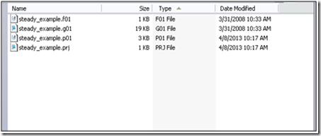
• .prj is the Project file. Contains current plan files, units and project description.
• .g01 is the Geometry file. Cross-sectional data, hydraulic structures and modeling approach data are stored here.
• .f01 is the Steady Flow file. Profile information, flow data and boundary conditions written in this file.
• For Unsteady Flow, .u01 is the flow file extension. This is where hydrographs and initial conditions are stored, as well as any user-defined flow options.
• For Quasi-Unsteady Flow (for a sediment analysis), .q01 is the flow file extension.
• .p01 is the Plan file. Contains a list of the associated input files, and all simulation options.

These are all text files and can be directly read and edited in a text editor. The following screenshot shows the input and output files after the steady flow model has been run. Note that some of these are only used by RAS as intermediate files during computations.

• .O01 is the Output file. Contains all of the computed results from the associated plan. This file is written in binary format and can only be read from the user interface.
• For Unsteady Flow, a .dss file is automatically generated as an output. This file contains time series data that is viewable by any program that can read dss files (typically HEC software).
• If your model links to a dss file for use as input data (e.g. inflow hydrographs, stage hydrographs, observed data, etc.), then that .dss file will be necessary to run the model and should be included in your group of files you send to a reviewer.
• .r01 is the Run file for steady flow analysis. Contains all of the necessary input data required for the RAS computational engine. The run file is created during the model simulation, and is not required to view final results.
• For Unsteady Flow, .x01 is the extension.
• .comp_msgs.txt is the Computational Message text file. Records the computational messages that pop up in the computation window. The messages file is not required to view final results, but can be useful in troubleshooting errors identified by RAS.
• .hyd01 is the Detailed Computational Level output file. This can be switched on in the Unsteady Flow Analysis window.
• .p01.rst is a Restart File (also called a Hot Start File, or Initial Conditions File). This option can be switched on by the user in the Output Control Options window. See the Hot Start post for more guidance.

For Unsteady Flow analysis, these files are categorized as “intermediate,” which means that they are not essential for running a model or viewing results, since they are recreated by RAS during run-time.

• .c01 is the Geometric Pre-Processor output file. Contains the hydraulic properties tables, rating curves, and family of rating curves for each cross-section, bridge, culvert, storage area, inline and lateral structure. This file is rewritten each time you change your geometry file.
• .b01 is the Boundary Condition file.
• .bco01 is the Unsteady Flow Log output file.
• .p01.blf is the Binary Log file.
• .IC.O01 is the Initial Conditions file.

If submitting your final model to a client or a reviewer, you will likely only send the necessary input files. Sending output files are optional, but will allow the reviewer to avoid rerunning the model on their end. Including the .c## files might be a good idea for larger models so that RAS can skip the pre-processing step. SEDIMENT ANALYSIS

• .S01 is the file extension for Sediment Data. This file contains flow data, boundary conditions, and sediment data.
• .SedCap01 is the extension for Sediment Transport Capacity data. When sediment transport computations are performed, RAS creates a set of intermediate files:
• .sed is the detailed sediment output file.
• .SedHeadXS01 is the header file for the cross section output.
• .SedXS01 is the cross section output file.
• .H01 is the Hydraulic Design data file.
• .H01.SiamInput is the SIAM Input Data file.
• .H01.SiamOutput is the SIAM Output Data file.

WATER QUALITY ANALYSIS

• .W01 is the file extension for Water Quality data. This file contains temperature boundary conditions, initial conditions, advection dispersion parameters and meteorological data. When water quality computations are performed, RAS creates a set of intermediate files;
• .bco is the water quality log file.
• .p01.wqrst01 is the water quality restart file.
• .color_scales is the file that contains the water quality color scale.

Remember that file extensions can be numbered from 01 to 99, and are assigned in the order that they are created.

Two-Dimensional modeling in HEC-RAS

Here's a quick sneak preview of what's coming in 2-D HEC-RAS.  Click either figure below to see an animation of the levee breach simulation.  More to come soon...

 

Extending your Cross Sections to High Ground?

Copyright © RASModel.com. 2013.  All rights reserved.

What are the implications of having a cross section that is too short and doesn't extend all the way out to the highest computed water surface elevation?  Does it affect the results?  Take this cross section for example. It is missing much of the left overbank (presumably).

Image courtesy of Adam Bohnoff

First of all, when RAS encounters this situation, it will automatically extend the last station elevation point vertically to the height of the computed water surface.  This adds a so-called "vertical wall" to the end of the cross section.  Additional wetted perimeter will be included for water that comes into contact with the "vertical wall". 

So what does this mean?  Well, you will be missing out on wetted area-possibly a LOT of wetted area.  Maybe it's negligible.  It's up to you to decide.  For typical rivers, the added wetted perimeter associated with the "vertical wall" will not make much of a difference in the results.  If you plan on mapping the computed flood plain in RAS Mapper, or in GIS using the GeoRAS extension, you'll miss out on some areas that should be shown as inundated. 

I see a few possible scenarios that you would need to consider.  Your course of action will depend on whether your model is steady or unsteady, and how much error you're willing to accept at this location:

1.  The missing wetted area is actually very small.  Either the maximum water surface elevation just exceeds the end point or perhaps there is a bluff just to the left of the first station elevation point that would contain all of the water.  In this case, you probably don't waste time getting additional survey data and leave the cross section as is, or you manually approximate in a station elevation point to capture the bluff. 

2.  There is considerable flow area that is missing, but it is so far out in the overbank or it's in a flow separation area and it can all be considered ineffective.  In a steady flow model, you can probably leave this as is.  Ineffective flow area is ignored in steady flow computations.  The answer will be slightly different if you extended the cross section and put in an ineffective flow trigger.  This is strictly due to the difference in quantified wetted perimeter.  For typical rivers, where the width is much greater than the depth, this will make little difference in your results.  For unsteady flow, there could potentially be a huge error in the results if you leave the cross section as is.  In unsteady flow modeling, ineffective flow areas are accounted for as hydraulic storage in HEC-RAS.  Hydraulic storage will attenuate the flood wave as it progresses through a system.  Omitting available storage can significantly affect both the propagation and attenuation of your flood wave.  I strongly recommend extending the cross section to high ground in this case. 


For steady flow, the differences in RAS will be very slight between these two options, limited to the wetted perimeter computed added at the vertical wall (ineffective flow assumes a frictionless boundary). In unsteady flow, these two options could produce VERY different results. 

3.  There is considerable flow area that is missing, and it is actively conveying flow.  In this case, steady, or unsteady, you'll want to extend the cross section to high ground.  Omitting this portion of your cross section will have a direct impact on the computed water surface elevation.  The degree to which depends on how much of the cross section area you are omitting, but it could be quite significant. 

So...how do we extend the cross sections?  In a perfect world, you'd have your survey crew go out and get you more points.  Unfortunately this cost money and takes time, frequently both of which you don't have an excess of when doing a hydraulic model study.  If your RAS geometry is already set up in GIS and your terrain model extends far enough laterally, you could simply extend the cross section cut line to the high ground and reimport into RAS.  Easy! 

However, if you do not have a georeferenced model and you can't get your survey crew out to the field in a timely (and cost-effective) manner, you can always approximate the extension of your cross sections using a USGS topo map. 

These "Quad" maps can be found for free on-line for any location in the US.  In fact, there are similar topography data sets for just about the entire world-available on-line for free.  The downside is that their resolution is quite inadequte for typical river modeling, and they don't include bathymetry (underwater topography).  However, for the purposes of extending your cross section to high ground, this can be an acceptable alternative to a physical survey. 

Simply find and download a terrain map that covers your area of concern.  Locate your existing cross section line on that map.  Then extend it to high ground, marking the locations where your cross section line crosses contour lines. Note the elevations, and the relative distances between contours, then manually enter that data as new station elevation points. 

Quasi Two-Dimensional Modeling in HEC-RAS

Written by Chris Goodell, P.E., D. WRE | WEST Consultants
Copyright © RASModel.com. 2013.  All rights reserved.

One of the limitations of HEC-RAS is that it is a one-dimensional model. Simply put, RAS assumes all flow moves along a singular dimension. For a given cross section, all of the flow is assumed to move either downstream, or all of it moves upstream, along the singular dimension (which can be defined as a polyline-does not have to be a straight line). The consequence of this is that there is only one water surface elevation (stage), and one total flow for a given time step at a given cross section. All of the other variables for a given cross section that you see in the profile output table, detailed output table, DSS, etc. are derived from the stage and flow values. This includes the velocity and shear stress distributions over a cross section, which can provide the appearance of a 2-dimensional analysis. But that is all based on a conveyance distribution over geometric segments of the cross section using that single water surface elevation and single total flow.

So why do I bring this up? First, it's always good to know ALL of the limitations of whatever model you're using to predict future outcomes. But I also want to demonstrate the "quasi-2-dimensional" capabilities of HEC-RAS. While planning a hydraulic study in an estuarine environment, you may immediately start thinking about which 2-dimensional model you want to use. But I've seen many great (and creative) applications of HEC-RAS in these 2-dimensional environments that produce very reasonable, if not accurate results.  In short, a quasi-2-d analysis in RAS requires you, the user, to understand up front the likely flow patterns in your study area. This is best accomplished by going out to the field and looking at your site, studying topographic and bathymetric maps, looking at aerial photographs, and simple common sense and experience. Once you've determined your perceived flow paths, all water outside of these flow paths should either be ineffective flow areas, storage areas, or even separate reaches.
  

Here’s an example of an estuarine environment on the Oregon Coast (Yaquina Bay). I haven’t modeled this yet, but if I were, here’s how I would approach my model setup:










1. Draw a stream centerline (blue in the figure) that represents the singular dimension of flow movement-i.e. flow will either move downstream or upstream along in the direction of this line. Cut cross sections at an appropriate spacing, making sure to cover all areas that could get wet during the simulation. Yes, the trib channel south of the main reach is not covered, but I’ll get to that in a second.

2. Define ineffective flow areas. These are areas that you will expect WON’T have flow actively moving along the singular dimension. Be sure to appropriately define expansion and contraction of flow as you draw in the ineffective polygons. All portions of your cross sections that fall within these areas should be set to be ineffective in your RAS model.  


3. Areas that could possibly have a different water surface elevation than the nearest cross section should be split out and modeled as an off-line storage area. Connect that Storage Area to the main reach using a Lateral Structure. You’ll have to come up with a stage-storage curve for the storage area, to be able to model it in RAS. This is a very easy and straight-forward exercise in GIS, as long as you have sufficient topographic coverage. Keep in mind, RAS uses the simplified level pool routing method for Storage Areas. Lateral Structures used for this application will not have an actual “structure” associated with it, so the discharge coefficient you use is very subjective. Typically values on the order of 0.5 to 1.5 are used. Calibrate this if you can.


4. Alternatively, you can model the tributary as its own reach, connected to the main channel with a junction. This will allow you to model it using the full dynamic St. Venant equations, giving a more physically representative answer in the trib. However, if movement of water through this reach is relatively slow (i.e. typical ebb and flood tides), a storage area will be fine-and easier!  You can get as complex as you want. There are no limitations within RAS to the number of storage areas, ineffective flow areas, lateral structures, and tributary reaches you use. Just keep in mind, the more complex you make it, the more difficult it will be to troubleshoot any instabilities.


The following video is a great example of a quasi-2-d application of HEC-RAS. This very complex model and the video were created by Gary Brunner at the Hydrologic Engineering Center.

HEC-RAS model of the Lower Columbia River Estuary-Courtesy Gary Brunner

Dealing with dry bed conditions for Creek/Spillway linked to a Reservoir Storage Area

Written by Daniel Christensen, P.E.     WEST Consultants
Copyright © RASModel.com. 2013.  All rights reserved. 

Our office ran into an unusual modeling situation recently.  Here is a description of the situation:  The project is a dam breach model, and the spillway for the dam diverts water to an adjacent basin.  The spillway is actually more like a canal (the spillway reach) that runs about a mile until it empties into the adjacent basin. The dam that impounds the main creek has a typical regulating outlet system that supplies water to the main creek, while the adjacent creek (supplied by the spillway) remains dry except for large flood events when the pool rises above the invert of the spillway.  The original unsteady model was constructed such that the creeks were modeled as separate reaches, both connected to a storage area representing the reservoir (see FIGURE 1 below).  Both the dam and spillway were modeled as an inline structures.  FIGURE 2 shows a close-up view of the spillway.

FIGURE 1 

FIGURE 2

  

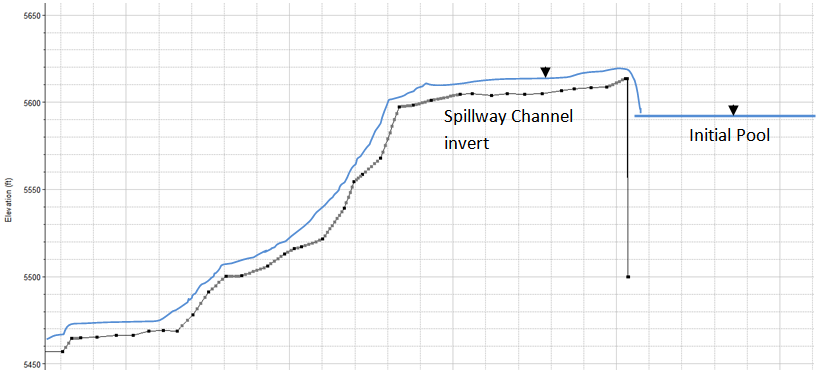
The problem we were presented with was: "How do we handle the dry-bed situation in the adjacent creek when the pool elevation in the reservoir is below the invert of the spillway?"  The starting reservoir elevation for the PMF/Flood Scenario dam breach was actually 20 ft below the spillway’s invert.   If you tried to the run the model with a boundary condition that was 20 feet below the main stream bed, the spillway reach would immediately go "dry" causing the model to crash (see FIGURE 3).

We had to get a little creative to resolve the dry-bed issue while still maintaining an accurate replication of the true geometry.  Instead of connecting the spillway reach to the reservoir storage area, we disconnected it and assigned a constant, low base flow to the spillway reach as an inflow boundary condition (100 cfs.  We knew the max flow for the spillway was 20,000 cfs so 100 cfs wouldn’t make a difference in the max stage in the creek).  This simple change fixed the dry bed issue in the spillway reach.  But we still need to provide a connection from the reservoir to the spillway reach, using the spillway crest as the hydraulic control.

FIGURE 3

To connect the storage area to the adjacent creek, we defined a lateral structure on the left bank that was 2 or 3 cross sections downstream from the top of the reach (see FIGURE 4).  The reservoir was defined as the lateral structure’s tailwater, and the spillway crest was used to define its weir embankment.  The weir coefficient was tested for multiple runs until the flow out of the lateral structure matched the spillway rating curve.  A final weir coefficient of 1.2 was used.  Also, to prevent the base flow (100 cfs) from flowing back into the reservoir when the pool elevation was lower than the spillway crest, “Flaps to prevent Positive Flow” were assigned to the lateral structure.  Keep in mind, positive flow is defined as the flow from the main channel that the lateral structure is associated with, to the tailwater (in our case, the spillway reach to the reservoir).  Therefore we only wanted to see "negative" flow.  Even though there were no "flap gates" in the spillway, using the "Flaps to prevent Positive Flow" feature, prevents any flow from going from the main channel to the storage area.

FIGURE 4

HTAB Problems with using the Drawdown Scheme for troubleshooting.

Written by Chris Goodell, P.E., D. WRE   |   WEST Consultants
Copyright © RASModel.com. 2012.  All rights reserved.

A very convenient way to troubleshoot instability problems with very complex models is the use of a hotstart run with a stepdown scheme.  Creating a stepdown scheme hotstart plan is covered in detail here.  In a previous post, I explained some problems with running the stepdown scheme when you have bridges.  Here I want to highlight problems you may run into with cross sections while running the stepdown scheme.
While drowning out the entire model to provide a high degree of numerical stability, you will be exceeding the maximum HTAB computation points, sometimes by several hundred feet/meters or more.  Technically, this is okay, since HEC-RAS will extrapolate the HTAB curves as needed.  However, extrapolation is done linearly off the last two HTAB points on the computed curve.  If the last two points of the curve happen to be at a location of discontinuity on the curve, bad things can happen.  Take for instance this computed HTAB curve of Conveyance vs. Stage:

It looks pretty good.  However, if you zoom in on the end point, you can see that there is a discontinuity in the curve. 

Not a big deal, since normally we are well below the last point on the HTAB plots.  However if you are running a step-down scheme, RAS will have to extrapolate off of the last two points when the model is “drowned” and you can see that there will be an overestimation of water surface elevation at the subject cross section during the stepdown process as shown below in the profile plot.  If the overestimation of stage is severe enough, the resulting “stairstep” could lead to numerical instability, causing your model to crash.
A quick fix to this problem is to just slightly change how the HTAB curves are constructed for the problem cross sections.  Simply remove the last point in the curve by reducing the number of points in the Cross Section Table Properties by 1 (in the example below, change 100 to 99). 

This will provide a much better linear extrapolation and get rid of the “stairstep” problem in the stepdown scheme. 

Of course a “seasoned” RAS modeler will recognize what is causing the discontinuity in the HTAB curve in the first place and could eliminate that problem by fixing the geometry, whether it be better definition of ineffective flow areas, levee markers, n-value breakpoints, etc.  However, the savvy modeler would recognize that the discontinuity exists at the end points of the cross section, well above the normal water surface elevation range.  Once the model is stable, there’s no need to spend time fixing this.  

Connecting a River to an Off-channel Storage Area using a Lateral Structure

Written by Chris Goodell, P.E., D. WRE | WEST Consultants
Copyright © RASModel.com. 2012.  All rights reserved.

An off-channel storage area in HEC-RAS can be a very useful way to simulate flooding in interior areas, adjacent ponds and lakes, urban areas next to rivers, green storage, or just about any area that you expect to flood but will be better represented as ponded water versus actively conveying water.  Connecting rivers to off-channel storage areas is done via lateral structures.  Although it is possible to use lateral structures and storage areas in steady flow modeling, typically lateral structures and storage areas are used in unsteady flow modeling, where quantification of storage and hydrograph attenuation are very important.

Here’s a simple example of using a lateral structure to connect a river to an off-channel storage area (this happens to be the LeveeBreach.prj project that comes with the HEC-RAS installation).

To begin, first make sure your cross sections are all included and correctly entered.  Then you draw in (or import from GIS) your storage area.  To do that, simply click on the Storage Area button on the top of the geometry schematic and start clicking points to define the perimeter of the storage area.  Double-click to complete the storage area.  Now you are ready to connect the river to the storage area.

Select the Lateral Structure button on the left side of the geometry schematic.    When you do this the first time, the following graphic will be blank, but in this case, the lateral structure (which is being used to simulate a levee) is already entered in.  The figure below shows the lateral structure in profile view.  The stationing plotted on the x-axis is the lateral structure stationing (which you will define in the Weir/Embankment editor).  It is NOT the same as the river stationing.

The River, Reach, and HW RS (Headwater River Station) define the location of the lateral structure in your system.  The upstream end of your lateral structure will be located at the HW RS (but can be shifted downstream of this station in the weir/embankment editor).  Notice that lateral structures are stationed from upstream to downstream (i.e. 0 is the most upstream point on the lateral structure).  The vertical lines in the graphic represent cross sections that are spanned by the lateral structure.  The vertical line that sits at station 0 is the HW RS.  The boxes on the bottom of the vertical lines represent the invert elevation of the respective cross sections, and the boxes on the top represent the end points of the cross section (on the side of the cross section that the lateral structure is located: left or right).  The red dots represent the bank stations of the respective cross sections.

Next, give a description for the lateral structure in the Description box and then define where its headwater position is.  You can place the lateral structure in either of the overbanks (left or right side) or adjacent to either bank station (left or right). 

The plan data Optimization button is just a shortcut to the plan file to quickly define whether or not you want to optimize the flow split over the lateral structure during the initial conditions run.  Typically you will want to optimize this if you have flow over the lateral structure at the beginning of the simulation.  If your initial conditions are below the lateral structure, leave this off.  The Breach button is a shortcut to the breach editor, if you want to breach this lateral structure during the simulation.

The “Tailwater Connection” is really the subject of this post-this is how you connect the river to the storage area.  Make sure you select “Storage Area” as your Type and then go choose the storage area you want to connect to by clicking the “Set SA” button.  Alternatively you could connect a lateral structure to another river/reach or you could connect it to nothing (send the flow over/through the lateral structure out of the system). 

There’s still work to be done to define the Weir/Embankment (if not already done), but the Storage area and the river are now connected via the lateral structure.  If you want to make sure you are connected, look at the points of the lateral structure on the geometry schematic.  If you see thin black lines connecting the end of the lateral structure to the storage area, then you know RAS recognizes them as being connected (sometimes you have so zoom in close to see the “connection lines”).

If you are having difficulty connecting lateral structures to rivers and/or storage areas, I highly encourage you to open up this example in HEC-RAS and have a look around.  Normally you will find the example projects in C:\Program Files\HEC\HEC-RAS\4.1.0\Example Projects.

The “4.1.0” might be different if you’re using a different version of HEC-RAS.  If you don’t see the example projects here, go to the Help menu item on the main HEC-RAS window and select “Install Example Projects…”