Pages

Friday, September 2, 2011

Overflow Gates

Written by Brian Wahlin, Ph.D.,  P.E., D. WRE | WEST Consultants
Copyright © RASModel.com. 2011. All rights reserved.
In modeling irrigation canals in HEC-RAS, a typical structure that is encountered is a check gate. Check gates are designed to back the water up behind them in an effort to keep the water level immediately upstream of these gates at a constant level. As the flow rates change in the canal, the gate openings on the check gates are adjusted (i.e. opened or closed) in order to pass the new flow rate while maintaining the water level upstream of the check at the desired elevation. Why go through this effort? Farmers usually get their water from these irrigation canals via orifices just upstream of the check gates. The flow through these orifices is dependent on the head (or the water surface elevation) acting on it. Since farmers want a constant flow rate delivered to their fields, the check gates in the main canal are adjusted when the flow changes to make sure the water level upstream of the check (and hence the rate of flow delivered to the farmers) remains constant.
Check gates can take a wide variety of forms, but typically they fall into two categories: undershot gates and overshot gates. Undershot gates are things like radial gates and sluice gates. As the name implies, water shoots “under” these gates. Inline weirs are typical examples of overshot gates. For these structures, water does not pass “under” the gate but instead flows over the top of the structure. Since many irrigation districts operate on limited budgets, it’s not uncommon to see an overshot gate made simply of several 2x4 wood boards that slide into groves in the canal walls. The irrigation canal operator “opens” these types of gates by manually removing one or more of the wood boards. In a similar manner, these gates are “closed” by adding one or more wood boards.
Modeling undershot gates has been straightforward in HEC-RAS for many years. You simply select whether you have a radial gate or a sluice gate and then enter the appropriate input data for the gate. The gate openings are then set through the flow editor-either steady state or unsteady state-depending on your situation.
Modeling overshot gates in HEC-RAS has been a little more challenging. Unlike the undershot gates, there really wasn’t a gate type that allowed water to flow over the top like a weir. Thus, you had to model overshot check gates using the geometry of the inline structure. An example is shown in the figure below. The four long white rectangles in the middle of the structure are undershot types of gates (in this particular case, they happened to be sluice gates). The two short white rectangles at the far right and the two at the far left (the ones with the open top) are overshot gates. Because in previous version of HEC-RAS, there wasn’t a particular “overshot” type of gate, you were stuck with coding these gates using the weir/embankment button. While this is perfectly fine for steady state mode where you only have one weir height setting, it becomes problematic if you run the model in unsteady mode and the weir height changes during the simulation. Because you have to model the weir as part of the geometry, there is no easy way to adjust the weir height as a function of time in unsteady mode.
clip_image001
Starting with HEC-RAS version 4.0, there is a new type of gate called an “overflow gate.” As the name implies, this type of gate allows water to flow over the top of the gate as shown in the schematic below. There are two types of overflow gates in RAS: open air and closed top. Both of these gates allow water to flow over the top of the structure. The difference is that the closed top gate is kind of like an elevated orifice. At some water levels, water will flow over a closed top gate like a weir. At higher water levels, the closed top gate will function as an orifice.
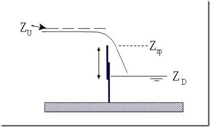
clip_image002
For irrigation canals, open air overflow gates are exactly what we need to model overshot check structures. To use this option, enter the inline structure information exactly as before. Now, select “Overflow (open air)” as the gate type. There are three types of weir shape methods: Broad Crested, Sharp Crested, and Ogee. For modeling irrigation checks, using the Sharp Crested option is probably most appropriate. With this option, there are three ways to enter the discharge coefficient for the weir equation: User entered coefficient, Rehbock equation, or Kindsvarter-Carter equation.
clip_image004
The gate opening is still set through the flow editor (either steady state or unsteady state). For overflow gates, the gate opening is now from the top of the gate rather than the bottom. The figure below shows a check structure modeled with open air overflow gates. As can be seen, the gate opening on the far left is 1.56 feet. But this distance is measured from the top of the gate frame rather than the bottom. Now, if you are running this model in unsteady mode and the gate opening changes (that is, another weir board is added or removed), you can reflect this in the gate opening boundary condition.image

Tuesday, June 21, 2011

Hotstarts and HTab Parameters at Bridges

Written by Chris Goodell, P.E., D. WRE | WEST Consultants
Copyright © RASModel.com. 2011. All rights reserved.


An advantage of running a step-down scheme hotstart run is the ability to spatially evaluate stability issues with difficult reaches. One of the elemental features of the step-down scheme is the artificially raising of the downstream boundary during the hotstart simulation to “drown-out” the reach and effectively create a very stable environment. During the hotstart simulation period, problem areas will identify themselves as the water surface elevation slowly lowers itself into a realistic solution. This is a great way to diagnose instability issues. However, if you have bridges or culverts, drowning-out the reach creates water surface elevations that are much higher than the normal water surface range you’d expect at those bridges, and a normal set of HTab parameters may not work well during the initial period of your hot start simulation. I’m speaking specifically about the “Head water maximum elevation” HTab parameter that is required at bridges and culverts. The figure below shows the problem that occurs with a normal headwater maximum elevation during a step-down hotstart run. Notice the flat pool downstream of the 3rd bridge, followed by a severe drop in water surface elevation. In a good hotstart simulation, the downed-out reach should show a consistently level water surface elevation. Ultimately this hotstart simulation crashed.

image

At first, it seems like an easy fix: Simply increase the head water maximum elevation for the affected bridge to an elevation around the “drowned-out” condition. In this case, I increased the head water maximum elevation to 350 ft, which is equal to the initial drowned-out elevation set at the downstream boundary. I make this fix and the profile looks good and the hotstart simulation runs to completion without errors. The figure below shows 6 profiles using the hotstart simulation with a step-down scheme. Notice the level pools as the water surface steps down to the true initial conditions.

image

Now that we have a good, stable hotstart run, switching to the real plan should be seamless, right? Actually, now that I’ve expanded the range of computation points for the rating curve at the 3rd bridge by using an artificially high head water maximum elevation, I’ve lost a lot of resolution in my rating curve for my real plan-particularly down in the range of real water surface elevations. Notice in the figure below that my expanded HTab curves go up to elevation 350 ft. Since I have a finite number of submerged curves, and points on the surbmerged and free flow curves, I have a loss in resolution in the range of realistic solutions (namely down in the 250 ft range).

image The real plan then crashes when the front end of flood wave reaches the 3rd bridge. The figure below shows error at the upstream end of the bridge that leads to the instability-and ultimately the crash.

image

There is actually a very easy fix. Simply change the headwater maximum for the “real” plan to a realistic maximum water surface elevation for that bridge. In my case, I reduced it from 350 ft to 270 ft. If you read through the hotstart posts in this blog, you’ll notice that I say any change in geometry will require a re-run of the hotstart plan, before running the real plan. To stabilize the hotstart plan, you’d have to put the headwater maximum elevation back to 350 ft, and then we’d be back to where we started. However, this is a rare exception to the rule. Luckily for us, changing the headwater maximum does not prompt HEC-RAS to want to re-run the hotstart plan. So we are free to change the HTab parameters at bridges for the real plan. Just make sure that if you DO re-run the hotstart plan, you change the headwater elevation back to the “drowned-out” condition (350 ft). Then “re-change” it to the realistic condition for your real plan (270 ft). It also helps to maximize the number of submerged curves, and the number of points on the free flow and submerged curves. This too provides more resolution. The figures below show the real plan solution with the more refined HTab parameters and the resulting profile plot. Notice the HTab curves are squeezed to a narrower range, providing more resolution. The difference in the solution on the profile plot is subtle, but makes all the difference between a stable and unstable solution at this bridge.

image

image

Monday, May 23, 2011

Modeling Junctions for Unsteady Flow Analysis

Written by Aaron A. Lee   | WEST Consultants
Copyright © RASModel.com. 2011. All rights reserved.

In the current version of HEC-RAS (v 4.1.0) there are two methods of modeling the hydraulics at a junction for unsteady flow. By default RAS selects the Force Equal WS Elevations (Forced) method, which forces the upstream bounding cross-sections’ water surface equal to the downstream water surface. This method may be adequate for some situations like high depths and shallow bed slopes, but can also cause major instabilities in your model if depths are too low and/or bed slopes are too steep. The alternative is the Energy Balance (Energy) method, which uses the energy equation across the junction to solve for WS elevations. The model presented in this post is part of a dam breach simulation and will demonstrate that there can be significant differences between the two methods. This simulation is a hotstart run which seeks to identify stability issues by starting the downstream stage artificially high, and slowly lowering it to the true solution over the run time. The river system in this model has a normal flow combining junction with a steep transition. Special attention will be paid to the steep transition, especially at low flow conditions. The Figure 1 below shows the 3D view of the model extents, which includes the Middle Reach, Tributary C and Lower Reach.


image Figure 1


For a normal flow-combining junction, the water surface elevations at the upstream bounding cross-sections are based on the computed downstream WS elevation. Longer lengths between the bounding cross-sections will generally make your results less accurate and less stable. By looking closely at the above figure you can see that the bounding cross-sections are spaced far apart, which corresponds to long junction lengths. The results for both methods are shown below in a series of profile plots. Figures 2a and 2b show the junction approximately halfway through the simulation. Figure 2a shows the Energy Balance method and Figure 2b shows the Forced Equal Water Surface method. The water surface is high enough that there are no differences between the two methods. For reference, Tributary C is the steeper of the upstream reaches.


image Figure 2a


image Figure 2b


Significant differences develop in Figures 3a and 3b as the downstream stage is lowered. At the same time-step, the two profiles are dramatically different. The Forced method produces a large drop at the junction (Figure 3b), while the Energy method produces only a minor instability (Figure 3a). The large drop (shown in Fig. 3b) occurs because RAS must balance the momentum equation from the upstream bounding cross-section at the junction (an unrealistically low water surface) to the cross-section immediately upstream. The only way to provide a balance is to overestimate the upstream WS elevation, which is why the profile for 3b is much higher than 3a. Notice the spike in the energy grade line. The same problem occurs for the Energy method, but at a much smaller degree.


image Figure 3a

image Figure 3b


Figures 4a and 4b show Tributary C only, just prior to the model crashing for the Forced Equal Water Surface method. There are obvious oscillations in the profile plot, which indicates a very unstable solution. As the stage is lowered downstream, the WS elevation at the junction also becomes lower. At a certain point the WS elevation at the junction approaches the invert for the upstream cross-section; and the model crashes. Figure 4b shows a zoomed in view of the WS elevation relative to the invert of the channel as the channel runs dry.

image Figure 4a

image Figure 4b


The best solution is to shorten the junction lengths as much as possible, which is done by adding cross-sections closer to the junction. By adding additional cross-sections you are decreasing the length over which RAS makes its calculations, which helps to remove the problems with low water surface elevations over a junction. If surveyed data is unavailable, then start by copying the most downstream cross-sections of the upstream reaches to a location closer to the junction. The positioning of these new cross-sections will be based on the judgment of the modeler, who should know the actual conditions of the river system. Make sure to adjust the downstream reach lengths and junction lengths accordingly.


In this example, cross-sections were placed within 20 ft of the junction. Junction lengths were changed from 573’ and 534’ to 35’ and 28’ for Tributary C and Middle Reach, respectively. In addition, cross-sections were added every 40’ on the steep section of Tributary C by interpolation. Figures 5a and 5b each show the profile plots for both the Energy and Forced method at the junction of Tributary C and Lower Reach.

image Figure 5a

image Figure 5b


By redefining the geometry around the junction the error is significantly reduced for both methods and the results appear stable. Both profiles are very similar in this case, showing only a slight difference in WS elevations. The dotted line-type represents the profile for the Forced method. It might not always be possible, or realistic, to place new cross-sections close to the junction. The Energy method allows this model to run to completion without the addition of new cross-sections, though the results appear to not be as good. The table below lists the WS elevations at the bounding cross-sections for each of the different plans: the initial Energy method, and the Forced and Energy method after adding additional cross-sections.


The initial plan has the geometry with the long junction lengths, which consistently calculates lower WS elevations than the plans with shorter junction lengths. Although the elevations were underestimated in the initial runs, they are still within 1 ft of the new profiles. For this model, the Energy method provides a stable solution at the junction without having to modify the geometry. However, given the steepness of Tributary C, the addition of cross-sections near the junction improved the accuracy and stability of the model output. Therefore, even though the Energy method can produce stable results for long junctions in steep reaches, adding more cross sections will improve the results.

Friday, April 1, 2011

Mixed Flow Regime Options – LPI Method

Written by Aaron A. Lee | WEST Consultants
Copyright © RASModel.com. 2011. All rights reserved.
By using the Mixed Flow Regime option for Unsteady Flow Analysis, RAS can better handle transitions from subcritical to supercritical flow. This option should be utilized only after determining that a mixed flow situation exists, which requires judgment from the modeler. One application where this could be particularly useful is dam breach modeling, or any other extreme and flashy flood event. Even though a model is stable there may still be small errors in the solution (caused by max. iterations). The Local Partial Inertia (LPI) factor may eliminate or reduce these errors, particularly if they occur when the Froude number is near 1. Figure 1 shows the Unsteady Flow Analysis window with the Mixed Flow Regime option selected. This post will focus on the LPI Filter, which is enabled when Mixed Flow Regime is selected by the modeler.


clip_image003


Figure 1. Unsteady Flow Analysis Window


Once the Mixed Flow Regime option is selected, additional settings can be adjusted to help stabilize the model. Navigate to Options, Mixed Flow Options. This window, shown in Figure 2, allows the user to adjust two inputs for the LPI factor.


clip_image007


Figure 2. Mixed Flow Options Window


For the unsteady flow computation scheme, RAS accounts for a local acceleration and convective acceleration (inertial terms) through the St. Venant equation of Conservation of Momentum. The St. Venant equations, and by extension, HEC-RAS, are designed to work best in gradually varied flow. Transitions from supercritical to subcritical flow (hydraulic jump), and to a lesser extent subcritical flow to supercritical flow, are rapidly varied flow situations. These are not gradual changes, in the hydraulic sense. Near critical depth (Froude number approaching 1) the convective acceleration terms can change very rapidly over a short distance (think of a hydraulic jump) and can lead to oscillations in the solution. These oscillations tend to grow larger until the solution goes completely unstable (HEC, 2010). The LPI factor systematically reduces these inertial terms to dampen the oscillations, helping to stabilize the model. The user can influence the magnitude of reduction by varying the two inputs in Figure 2.


The first input, m, is the exponent for Froude number reduction factor. Its default value is 10 and ranges from 1 to 128. Adjusting m will change the shape of the curve on Figure 2, thus influencing the rate of reduction of the inertial terms. You can see that by making m smaller there is an earlier and more direct reduction in the inertial terms, with respect to the Froude number. Increasing m can make the model more accurate but increases the likelihood of numerical instability.


The second input, FT, is the Froude number threshold at which the LPI factor is set to zero. In other words, if the calculated Froude number at the current cross-section is larger than FT the inertial terms will be eliminated from the computations at that cross-section for the current computational time step. The default value is 1. Making FT smaller will improve the stability of the model, but will also reduce the accuracy. A larger FT can make the model more accurate, but increases the likelihood of numerical instability as the inertial terms will be more sensitive to fluctuations in Froude number.


A good place to start is to run the simulation with the default values


and see what the profile looks like. For this flume example, the model ran without reporting any maximum water surface errors. The profile for the default LPI inputs is shown in Figure 3.


clip_image010


Figure 3. Profile Plot, Default Values


Next, a value of 1.6 was chosen for FT. This simulation yielded small maximum water surface errors, but had maximum iterations at various locations. The value of m was left unchanged. Figure 4 shows the results.


clip_image013


Figure 4. Profile Plot, Increased Froude Number Elimination Threshold


Even though the errors were small, instabilities could be seen in the downstream end. Notice the instabilities around the transitions between the flow regimes. The value of m was reduced from the default of 10 to 7 in order to improve the stability of the model. Figure 5 shows the profile for reduced m and increased FT. The modeler should choose the largest values of m and FT that produce a stable model. However, check the results to make sure that the output is reasonable. Notice how the transitions between flow regimes are much better defined in Figure 5 then the default setup shown in Figure 3. That’s because the default LPI parameters (m = 10 and FT = 1) provide dampening of the results. Though Figure 3 looks very stable (and it is), Figure 5 (m = 7 and FT = 1.6) is both stable and (by my engineering judgment) more accurate. Also, notice how the slight increase in energy (green dashed line) is less in Figure 5 versus Figure 3. An increase in the energy elevation in the direction of flow is an indication of error in most cases. Further adjustment of the LPI parameters may help to eliminate the error in the energy grade line, while still producing a stable solution.


clip_image015


Figure 5. Profile Plot, Increased Froude Number Elimination Threshold and Decreased Exponent ,m

Wednesday, March 9, 2011

More on HTab Parameters

Written by Chris Goodell, P.E., D. WRE | WEST Consultants
Copyright © RASModel.com. 2011. All rights reserved.

I’ve mentioned this a lot in this blog, but I’m finding more and more that a good, solid definition of your HTab parameters up front will go a long way in helping construct a nice stable unsteady flow model in HEC-RAS.

First, let me recap how they work. In unsteady flow, HEC-RAS will convert the geometry of cross sections into a set of curves defining relationships between hydraulic parameters and stage (it does the same thing for bridges and culverts, but we’ll save that for another post). These hydraulic parameters include conveyance, flow area, storage area, and top width. This is done for the main channel, overbanks, and for the total cross section. Storage area in this case represents any ineffective flow areas in the given cross section. The figure below shows the conveyance HTab curve for a cross section.

image

These curves (actually the paired data that creates them) are used by HEC-RAS during the unsteady flow computations. Rather than re-computing the hydraulic parameters at every time step, RAS can simply pick the value off the chart. Because these curves are defined by a number of discrete points, RAS usually must interpolate to grab a value in between points. RAS does this linearly. Herein lies the problem that can lead your model to errors and instabilities.

Notice how at the lower stages, there is a significant curvature to the conveyance relationship in the above figure? A linear interpolation in this range can be quite wrong if the resolution of points is too coarse. Notice how when I zoom in to a rather coarse Conveyance HTab curve, it becomes obvious that in between points, linear interpolation is going to give me a bad answer. This is why a good definition of HTab points is particularly advantageous when running at low stages.

image

Start by maximizing the number of HTab points for you cross sections. HEC-RAS allows up to 100. The grey horizontal lines in the figure below represent computation points at different stages. I know what you’re thinking. “Won’t that many points on every cross section really slow down the computations?” Well, that may have been the case years ago, but computers are so fast now, that you’ll probably never notice the difference. Furthermore, the development of these curves is only done once, during the preprocessing part of the computations. As long as you don’t change the geometry, RAS won’t have to recompute the HTab curves.

image

Then make the computation increment as small as possible to squeeze all the points together. You only need to extend your HTab curves to contain the maximum computed water surface.

image


Finally, go to the Stating El. column and click the button “Copy Invert”. Notice in the figure below there is a gap between the invert of the channel and the first computation point which is set 1 ft above the invert of the main channel. image This is the default starting computation point in RAS (well, not completely true). If you check the 2nd figure up above, you’ll see that there actually was a computation point at the 0 depth point (the invert). That’s because RAS will still compute the 0 depth point, but then the next computation point, by default, is 1 ft (0.3 meters in SI Units) above the 0 depth point. From there on up, RAS will space the computation points based on the increment you define. To get more points between the invert of the main channel and 1 ft (0.3 m) above the invert, you have to set your Starting Elevation to the invert. That’s why it’s always a good idea to click “Copy Invert” and make sure that your Starting Elevation is the same as your “Chan Min” value. That way, the small computation increment is started from the channel invert, not 1 ft (0.3 m) above the channel invert.

image


I was recently informed that in the next release of HEC-RAS (version 4.2), the default starting point for HTab computations will be 0.5 ft above the invert (0.15 m?). This will improve things somewhat, but it still may be necessary to “copy the invert”, particularly if you have very low stages in your simulation.

Tuesday, December 28, 2010

How to Create a Hotstart File in HEC-RAS for Dam Breach Analysis

Written by Aaron A. Lee   | WEST Consultants
Copyright © RASModel.com. 2010. All rights reserved.
While running unsteady flow simulations in HEC-RAS instabilities may occur when transitioning from the automatically created initial condition file to the first computed time step. These instabilities can be caused by mixed flow conditions, flow splits, or poorly defined initial conditions. A hotstart is another option available for defining initial conditions for the project model. This article presents one technique for setting up a hotstart run to help with initial conditions problems and to troubleshoot problem areas in your project model.

This is done by creating a new plan, using a flow file with a constant discharge as the upstream boundary, and a stage hydrograph as the downstream boundary over a 24 hour period. Typically 24 hours is long enough, but you may find that a longer hotstart period is required. The downstream boundary water surface elevation is defined artificially high, and over the simulation it is gradually reduced until it reaches the true starting depth for your project model. At this point the hotstart file will be written by HEC-RAS. In HEC-RAS lingo, the term “hotstart file” is used interchangeably with “Restart File” and “Initial Conditions file”.

STEP 1. Create a new flow file by opening the current unsteady flow file and navigate to File, Save As, and name it “hotstart”. Once saved, change the upstream boundary condition by selecting Flow Hydrograph under the Boundary Conditions tab. Change the discharge to a constant flow equal to that of the first timestep for the 24-hr period. In this example, shown in Figure 1, the entire Flow column should be modified to contain 155 for the full 24-hr simulation.

image

Select Stage Hydrograph as the downstream boundary condition. The beginning stage should start at an artificially high elevation - somewhere near the invert of the upstream-most cross section. The final elevation at the end of the 24-hr simulation should be equal to the starting downstream water surface elevation of the project plan. Once these values are added into the Stage column, use the Interpolate Missing Values button to add the missing elevations.

The elevation at each time interval should gradually decrease. This makes it easier for the modeler to observe problems as they occur, and where they happen in the model. For this example, the starting elevation is 820 ft and the final elevation is 637.25 ft. This is shown in Figure 2. Save the “hotstart” flow file.

image STEP 2. Navigate to the Unsteady Flow Analysis window and save as a new plan named “hotstart plan”. Name the short ID as “hotstart”. This will create a new plan that will be used to define the initial conditions for the project plan. Under the Unsteady Flow Analysis window select the Ending Date and Time to 24 hours after the Starting Date and Time (or whatever time frame you want to use-just be sure it is consistent with the hotstart flow hydrograph and stage hydrograph you created in Step 1).

STEP 3. The next step is to set up the model so that the hotstart file will be written. Under the Unsteady Flow Analysis window navigate to Options, then Output Options. Figure 3 shows this window.

image

Check the boxes that write the initial conditions file at the Fixed Reference of the hotstart simulation ending date and time. At the end of the specified simulation time (24 hours) HEC-RAS will automatically write the initial condition file. The final step is to ensure that the hotstart plan is using the correct geometry file, and the created “hotstart” flow file. Once the plan is completed and saved, compute the Hotstart simulation.

STEP 4. The profile plot should be reviewed for problems with the hotstart model. This will indicate areas that may cause problems in your project model. Over the course of the hotstart simulation, as the water surface drops into place along your bed profile, look for hints of instabilities. If you hotstart simulation crashes, you’ll know exactly where to investigate-the intersection between the artificially high horizontal pool and the bed profile at the time of the crash. To use the hotstart file as your initial conditions, go to the Unsteady Flow editor of your project plan. Click on the “Use a Restart File” box and browse for the initial conditions file. This file will have an extension that indicates that hotstart plan number that created it, the simulation time (day-month-year) when it was created, and .rst. In this example, it should look like:

Workshop4.p03.10NOV2006.rst

*Warning-If you make a change to the geometry in your project model, you’ll have to re-run your hotstart simulation. However, once everything is set up, this is very easy to do. Simply open the hotstart plan and run it. Then open the project plan and run it.

Friday, October 22, 2010

Some useful debugging tools

Written by Chris Goodell, P.E., D. WRE | WEST Consultants
Copyright © RASModel.com. 2010. All rights reserved.

Recently I’ve had some real difficult models to set up and run. Some real beasts. And some of these take hours to run. As you can imagine, when one of these models is crashing, strategies for effectively diagnosing and fixing errors become very important. You don’t want to “chase” problems in models with 2 hour run times. You’ll never get your model stable. You need to be able to diagnose the problem and come up with a confident fix, while minimizing the time spent running the model to “try out” possible fixes.

Here’s a real useful tool that has recently been added to HEC-RAS.

image

In the Runtime Computational Options, you have the option to “disregard” Lateral Structures, Storage Area Connections, Breaches, and Pumps in the computations. Let’s say you turn off lateral structures, rerun your model and it runs fine.

image

Then you know that there is a problem with one or more of your lateral structures. Simple diagnosing tool-but very effective.


Also, I’ve been using the Computation Level Output a lot. By checking this box on the Unsteady Flow Analysis window, you are able to look at some select output parameters at every computational time step interval. These parameters include water surface elevation, flow, and lateral inflow. You can view two types of plots: a spatial plot and a time series plot, by going to the “View” menu item on the main RAS window.

image

The first two are very useful, and at a computation interval level, can show you things that just won’t show up on the detailed output profile plots. However, the ability to monitor lateral inflow, graphically, and at the computation interval level, is a powerful way to determine when and how much discharge is entering a given reach laterally (via lateral structures from other reaches or storage areas).

image This is a common source of errors that can lead to instabilities in complex HEC-RAS models, and aside from this plot, I don’t know of another way to graphically see this.