Pages

Monday, December 28, 2009

Latest DSS-Vue Plug In

Posted by Bill McDavitt:


"(DSS-Vue) now allows users to injest 1 hour data (sometimes the gage even has 15-minute data) from the USGS Instantaneous Data Archive using the latest plug-in, just released in November. I've been able to work on some projects that happen to have gages very nearby, which I realize is a bit of a rarity. Nonetheless, with 15 mintue data in a DSS file, making an unsteady flow model using data for a particular storm flow can be done with relative ease and minimal additional time spent.
If a user is comforatable scaling/adjusting the gage data for their non-gaged site, HEC has an Excel tool whereby the flows could be modified in Excel and then repackaged into a DSS file."

2009-A look back in HEC-RAS

Written by Chris Goodell, P.E., D. WRE | WEST Consultants
Copyright © RASModel.com. 2009. All rights reserved.

2009 was a very interesting year for HEC-RAS. A beta version of 4.0.1 came out which included a new Floodplain Mapper (RAS Mapper). This looks like a great start to realizing a fully functional HEC-RAS model with built-in GIS capabilities. Also, Modified Puls Routing for steep streams and a new and improved method for computing at junctions in unsteady flow were added. Sediment Transport continues to improve, and I know that HEC is currently working on a two-dimensional component to HEC-RAS (both in series and in parallel). More water quality functionality was added (though I admit to not having worked with this too much). All great stuff. From what I hear, version 4.1 will be out soon. Keep checking back on the HEC website often.

As for the first full year of the HEC-RAS Bloggery, I was pleased with the response and readership. We talked about the limitations of RAS, failing bridges, Cross section spacing, minimum flow requirements, Htab strategies, cross section interpolation, RAS precision, bridges and culvert strategies, sediment transport issues, and possibly the most popular topic of late...n values in steep streams.

Thanks to all for reading and responding. Please let me know if there are ways to improve the HEC-RAS Bloggery, or any topics you would like me to write/comment about. Also, I want this to be more of a public blog posting site. So if any of you have articles you've written that you would like to post in the HEC-RAS bloggery, feel free to email to me (Chris G.) and I'll post them up. I would like to hear about other's experience with Water Quality in RAS, Sediment in RAS, Channel Modification, more on n values in steep streams, or just something you've done with HEC-RAS that was really cool.

Thanks and all the best in 2010!

Tuesday, December 15, 2009

n-values in steep streams

Written by Chris Goodell, P.E., D. WRE
Copyright © RASModel.com. 2009. All rights reserved.

What is a good range of n values for a typical river or stream bed? 0.03?0.045? What about a mountain stream? 0.05? 0.07? Jarrett has a very simple formula that serves as a good check on n values in mountain streams. He developed his equation from 75 observations of streams in Colorado. His streams were composed of bed material ranging from cobbles to small boulders. Range of energy slopes were 0.002 ft/ft to 0.09 ft/ft and range of hydraulic radii were 0.5 to 7 ft.

Jarretts equation is: n = 0.39*(S^0.38)*(R^-0.16), where S is the energy slope and R is the hydraulic radius of the stream (in US Customary length units of feet).  (*Note-the original post had mistakenly listed the equation as 0.47*(S^0.38)*(R^-0.16).  That was incorrect.  The correct equation, as published in "DETERMINATION OF ROUGHNESS COEFFICIENTS FOR STREAMS IN COLORADO" by Robert Jarrett is n = 0.39*(S^0.38)*(R^-0.16).  Sorry about the mistake!)

Using his range of energy slopes and hydraulic radii, you could compute n values from 0.032 to 0.21. Yes, that's 0.21!!! I have had discussions with many class participants of mine who indicate that indeed they are finding n values much higher than traditionally what have been used. We're talking as high as 0.12 to 0.15 in some cases. This definately fits within Jarrett's confines. Partly to blame in this underestimation of n values in steep mountain streams would be the very popular table of n values in Chow. Chow lists mountain streams as having n values from 0.03 (gravels, cobbles, and a few boulders) to 0.07 (cobbles with large boulders). Also, another popular n value predictor, Barnes (USGS), lists it's highest n value stream as Rock Creek near Darby Montana, with an n value of 0.075. Rock Creek is composed of boulders with a d50 of about 220 mm. However, this was measured during a flood. It is likely that the n value is much higher at lower discharges where the bed irregularities have a greater impact on the overall roughness.

I like to use Jarrett's equation whenever I'm dealing with steep mountain streams that fall within (or close to) his experimental range. A little secret here: higher n values helps to stabilize unsteady flow models!

I'm curious to know if anyone out there has comment on this topic. I'd like to know what kinds of n values you all are coming up with for steep streams.

Monday, October 26, 2009

Dam Breach class-Portland, ME

I'm heading out to the HEC-RAS Dam Breach class in Portland, Maine tomorrow. Glad to see that enrollment in our classes is making a rebound. Mt last 2 classes were cancelled due to low attendance.

Thursday, September 17, 2009

Sediment Mass Plot/Invert Change Issues

Written by Chris Goodell, P.E., D. WRE | WEST Consultants
Copyright © RASModel.com. 2009. All rights reserved.

A very common "head-scratcher" for sediment modeling is the situation where your mass plot is showing a lot of accumulation of sediment at a given cross section (mass plot curve rises with time, indicating deposition), but the channel invert shows no change over the same time period. Usually this is due to the placement of the moveable bed limits.

Keep in mind the spatial plot only shows the minimum elevation node for each cross section. As a result, a depositional zone may not be captured correctly in that plot, if the mobile bed stations are missplaced. This example shows the mobile bed limits placed low in the channel. As the bed aggrades, the low point moves out to the mobile bed limit and its elevation remains constant throughout the simulation. The Sediment Spatial plot will indicate the cross section is stable, when in reality it is depositing a lot of sediment. A check of the mass plot will help to figure this out. One solution would be to move the bed limits out onto the banks, so that the minimum cross section point moves up with the deposition . Also, you could move the bank stations inside of the moveable bed limits, if that is acceptable to your conveyance distribution (remember, the minimum bed elevation is reported inside the bank stations). Or, you could leave it as is, and just recognize that the channel invert plot is misleading.

Tuesday, September 15, 2009

Initial Reservoir Elevation-Pilot Flow

Written by Chris Goodell, P.E., D. WRE | WEST Consultants
Copyright © RASModel.com. 2009. All rights reserved.

A common question when modeling reservoirs with cross sections (dynamic routing) is how do I get my reservoir elevation to start where I want it to? Using Pilot Flow at your inline structure is a very easy way to guarantee your water surface elevation starts exactly where you want it to. First, you want to make sure that the pilot flow is equal to your initial conditions flow into the reservoir. Now, if you only did this, the reservoir would never fill up, as it would be passing everything that came into the reservoir, right out of it (no storage). To get your reservoir where it should be, go to the unsteady flow editor, and select Options...Internal RS Initial Stages. Pick the cross section just upstream of the inline structure and assign it the starting water surface elevation you desire. Now keep in mind this will only set the initial water surface elevation in the reservoir. For the remainder of the simulation, the reservoir level will move based on inflow, outflow, and storage (as it should). However, pilot flow is constant throughout the simulation. It does not change with reservoir level. Therefore only use this technique if the pilot flow is small compared to the flood discharges you are looking at. A great application is a dam breach flood where the discharge from the dam breach will be orders of magnitude greater than any pilot flow you use.

Monday, August 3, 2009

Problems with bridges and culverts.

Written by Chris Goodell, P.E., D. WRE
Copyright © RASModel.com. 2009. All rights reserved.

(Thanks Eric for the topic). It's very common for HEC-RAS models to show inconsistencies around crossings (bridges and culverts). Usually, 1 of 3 things is going on here: 1. Bad geometry-either incorrectly entered, or poorly defined. 2. Numerical errors. 3. The results are actually correct and can be explained.
For the first case, "bad geometry", here's a technique that can be used to help spot sources of problems. Create and evaluate the hydraulic property plots for the crossing. If you are running unsteady flow, this is done for you during the geometry preprocessing task. If you are running a steady flow model, you can create an unsteady flow plan and just run the geometry pre-processing task (you don’t need to run the computations or the post-processing. Once that’s done, on the main RAS window, go to View…Hydraulic Property Plots. Click Type…Internal Boundaries, and you’ll see the family of rating curves for your crossing. Here you’ll want to examine the curves and look for any abrupt changes, or discontinuities, particularly in the range of flows/depths where you are seeing the discrepancy. Typically you see problem areas where RAS changes equations (i.e. going from low flow to pressure flow, or pressure flow to pressure and weir flow), or when ineffective flow triggers turn off/on. Also, keep in mind that the equations for culverts are very different from those used for briges in HEC-RAS.

Take the following example, in the figure below. First of all, I always like to open up the bridge plot along side its htab plot (make sure the vertical axis is consistent) so that I can graphically explain any discontinuities in the htab curves. This example shows a significant discontinuity at around 10,000 cfs (you can click on the figure above to get a better view). It's very obvious from looking at the plot that this is the range at which the flow transitions from low flow to pressure flow and then on to pressure and weir flow. Also, notice that the ineffective flow triggers turn off in this range. It appears that the creater of this model tried to lessen the impact of the ineffective flow areas instantaneously turning effective by significantly raising up the n-values in the overbank. Not a bad technique, but obviously didn't completely solve the problem.
Things you can tweak that may provide more sensible results and a better set of Htab curves are:

-Coefficients (bridge and culvert coefficients).
-Ineffective flow areas upstream and downstream of the crossing.
-Bridge modeling approach.
-Placement of cross sections. Sometimes if they are too far from the crossing, or to sparsely spaced leading up to the crossing, it can cause these types of problems.
-Consider modeling a bridge as a culvert, particularly if it has a very deep deck and small relative opening. Likewise, consider modeling a culvert as a bridge, particularly if it has a very large opening, relative to the deck thickness (conspan culverts are good examples).

If the problem is only a very small discrepancy in upstream head levels, a refinement of the computation tolerances might yield better results. For example, let's say you are trying to provide a "no-rise" condition, and you feel that there should be no rise (i.e. new bridge opening is bigger than old bridge opening with a higher low chord). However, you're results are showing a 1 to 2 hundreths of a foot of rise for the new bridge. This is most likely numerical issue and a refinement of the computation tolerances might yield better results.

Tuesday, July 28, 2009

RAS Mapper


Written by Chris Goodell, P.E., D. WRE
Copyright © RASModel.com. 2009. All rights reserved. 


*Update:  This post is outdated now with the release of HEC-RAS Version 5 and higher.  RAS Mapper is now completely different.  


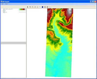
So Riley and I recently gave this a thorough run through. After a few bugs were fixed up, it works quite nicely. The key here is you have to have a terrain model that is spatially and vertically consistent with your RAS geometry. Once you've successfully run your model, and you have a terrain model in the form of a floating point grid format (*.flt), you are ready to map within HEC-RAS (i.e. no ArcGIS required).

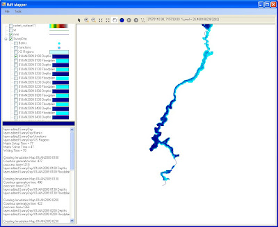
On the main HEC-RAS window, go to GIS Tools...Floodplain Mapping. I know, there is no "GIS Tools" menu item on the main HEC-RAS window. In the next release (4.0.1) there will be. This will bring up the RAS Mapper. It looks like a very basic version of ArcGIS. By default you'll see your river and cross sections plotted in plan view. One of the tools allows you to define a projection, but if everything is consistent, you can bypass this and go right to mapping. Here, you'll be able to bring in your terrain model. This is seriously way too easy. Next you simply click on the profiles you want to map and click "Generate Layers." There you'll see all of the floodplains and associated depth layers that you requested. The only thing missing...animation of the RAS Mapper. Maybe if I ask real nice they'll put that in.
Floodplain Map

Depth Map.

Tuesday, July 21, 2009

Other New Features in version 4.0.1

Written by Chris Goodell, P.E., D. WRE | WEST Consultants
Copyright © RASModel.com. 2009. All rights reserved.

Here's a brief summary of some of the other new features that will be debuted in the new 4.0.1 release:

1. Geometry Window...Options...Main Channel Manning's n Value Compositing. I believe this was available elsewhere to a limited degree before. Now you can change the Compositing Slope Criteria or choose to not autmatically composite.


2. Geometry Window...Tables...Contraction/Expansion Coefficients for Unsteady Flow. Not sure what this is about. My understanding is that the C&E losses were built into the unsteady flow equations. I'll have to check into this.
3. Geometry Window...Tables...Minor Losses. Apparently you can add additional losses to a specific cross section. This is set up to take a Minor Loss Coefficient that I'm guessing is muliplied by the velocity head at every time step for the additional loss. Maybe to be used for tunnels or pipe networks (using cross sections with lids, or priessman slot...).
4. Unsteady Flow Analysis...Options...View Runtime messages file. Awesome! Gone are the days where you have to rerun your 10 minute-long simulation just to find out where it crashed because you inadvertantly closed the computation message window. RAS now stores this info in a log file. By selecting this option, you can view that log file. Great add!

5. Unsteady Flow Analysis...Options...Automated Roughness Calibration. This is HUGE if it is what I think it is. I haven't had a chance to try it out, but is appears you set up flow roughness factors and add in some observed stage gage data (unsteady flow editor options), then in this window, you can specify some calibration parameters. RAS will then automatically adjust your Manning's n flow roughness factors to match the gage records. Very cool.

Not sure when this new version will be officially out for the public to download, but hopefully soon. Keep checking back at the HEC website.

Tuesday, July 7, 2009

New Features 4.0.1 Part 3...Modified Puls Hydrologic Routing

Written by Chris Goodell, P.E., D. WRE | WEST Consultants
Copyright © RASModel.com. 2009. All rights reserved.

This will be a very useful feature for those pesky dam breach unsteady flow models (or any very dynamic unsteady flow model) with steep sections of reaches and low depths. By designating a portion of your reach to be solved using the Modified Puls Hydrologic routing technique, you are removing a common problem with unsteady flow solution scheme used-it is very sensitive in steep, shallow reaches, especially during the rising limb of the breach hydrograph.

In the previous version of RAS, we could sometimes model short steep reaches with inline structures, but that always felt a little like cheating to me. Plus, what discharge coefficient do we use? For longer steep reaches, we would have to run a separate HEC-HMS model of the affected reach, then import those results to steady flow RAS to map it. That was kind of painful, but occasionally necessary. Now all of it is built into HEC-RAS, so switching to a different model is no longer required.

First thing you have to do is set up a steady flow run with multiple profiles (flows). These flows should encompass the full range of expected flows in your unsteady flow run, from low initial flows to the peak of the flood event. I found that this feature did not work when it had to extrapolate. Keep in mind that the more steady flows you include, the better storage/outflow relationship can be established.

In the geometry editor, go to Options...Hydrologic Unsteady Routing, and you'll get the following window. Here you simply select regions where you want to apply the modified puls routing and then import the storage-discharge relationship (RC's) from the steady flow profiles for each region. Each cross section within a region will be treated as an individual Modified Puls "Reservoir". Make sure you select the "Use Modified Puls Routing" checkbox, and then you can compute the unsteady flow run.


Thursday, June 25, 2009

New Features 4.0.1 Part 2...Junctions

Written by Chris Goodell, P.E., D. WRE | WEST Consultants
Copyright © RASModel.com. 2009. All rights reserved.

Up until now, unsteady flow HEC-RAS uses a very simplistic method for handling juctions. It simply projected the water surface elevation of the downstream cross section to the two cross sections upstream of the junction. For shallow, deep systems, this worked fine-no problems. However, if you tried to model a steep reach with shallow depths you run into a host of problems at junctions. I've blogged about this problem before and provided examples of ways around to work around it. However, in the new version soon to be released (4.0.1) HEC has taken care of this problem and it works quite nicely.

In the Junction Editor, you'll notice that there is a new option for unsteady flow.

You can either keep the original, simplistic computation mode, or require RAS to perform an energy balance around the junction. I'm assuming HEC left the original "Force Equal WS Elevations" method in as the default so that your results will remain the same when you upgrade to 4.0.1. I don't believe that the new method is computationally burdensome, so I would expect that for new models, you'll want to check the "Energy Balance Method", particularly if you'll be working with steep reaches and/or shallow depths.

Monday, June 15, 2009

New Features 4.0.1

Written by Chris Goodell, P.E., D. WRE | WEST Consultants
Copyright © RASModel.com. 2009. All rights reserved.

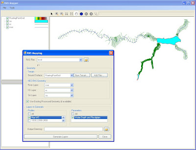
I just got a preview of the new release of HEC-RAS 4.0.1. Even though the release id would suggest it's a minor release with only bug fixes, there are (at least) two major additions to the software: Today I'll show you a little bit about the RAS Mapper. This will allow you to take your steady and unsteady flow results and map the floodplains directly within the HEC-RAS environment. In other words, you won't have to export into ArcGIS (at least not initially). The RAS mapper is a lot less complex than ArcGIS, but includes features like adding layers, defining projections, and inundation mapping. Inundation mapping requires a terrain model in floating point grid format (*.flt). These are very easy to create within ArcGIS. To finalize a map and smooth out the boundaries of the floodplain, you'll probably still have to go to ArcGIS. However, now you can just bring in your shapefile created in the RAS Mapper, as opposed to going through the PostRAS procedures in GeoRAS. Unfortunately, for now, GeoRAS is still required to create a geometry file from GIS.

From the look of the new RAS Mapper, it appears that you simply select the profile you want to map, specify your terrain model, give it an output directory and click "Generate Layers".
Now I have to get a floating point grid set up so that I can give this a try...

Wednesday, June 3, 2009

Energy Grade Line Problems

Written by Chris Goodell, P.E., D. WRE | WEST Consultants
Copyright © RASModel.com. 2009. All rights reserved.

Why do you sometimes see the water surface elevation and the total energy increase in the downstream direction? The energy grade line should always slope downhill. Water surface doesn’t necessarily have to though (i.e. hydraulic jumps, transition from narrow cross section to wide cross section). In this case, I’m not sure what the problem is without seeing the model firsthand, but the EGL indicates localized errors. This usually occurs from either not enough cross sections, or HTAB computation points that are too coarse, or the computation points don’t go low enough in the cross section. Try maxing out the number of HTAB points for each cross section, and decrease the increment as well. Also, use the invert of the channel as the starting computation point (there’s a button to do that automatically). Run the model. If there are still some problems, try interpolating some cross sections in the areas where there is increasing energy. Also, turning on the critical depth variable in your profile plot can help to explain what’s going on.

HEC-RAS Help or Troubleshooting

Written by Chris Goodell, P.E., D. WRE | WEST Consultants
Copyright © RASModel.com. 2009. All rights reserved.

I wanted to take the opportunity to throw out a few resources for finding HEC-RAS help and troubleshooting models. First off, unless you work for the Corps of Engineers, HEC can not offer technical support to you. They are happy to receive bug reports from anyone, but for help on methods, concepts, and general how-to's, they are just not equipped to handle it. You may be surpised at how small (in #s of employees) HEC really is. Anyway, when I'm looking for help, I usually consult the manuals first. Now-a-days, you can get to the manuals directly though the Help menu item in HEC-RAS. These manuals are very well written. It is quite possible that the answer to your question is already documented in the manuals. Also, check the Release Notes, and "What's New" documents on the HEC web site (http://www.hec.usace.army.mil/).

If that doesn't help, search this blog, using the search tool on the right side bar.

Still no luck? Try a forum dedicated to HEC-RAS. The Boss website has a great forum for HEC-RAS (among other software and topics). It has been around for a long time and has countless postings. Be careful though. I'm not sure how well this forum is moderated and I've seen some very bad suggestions and just completely erroneous replies. http://www.bossintl.com/forums/hec-ras/

This is partly the reason I started the HEC-RAS Bloggery Forum. Although it it very new and there's not a lot on there yet, I moderate all postings and replies. If something is posted that is not accurate, it will be corrected or removed.
http://forum.rasmodel.com/user/categories.aspx

Still no luck? There's always the option of getting professional consultation and technical support from an expert in the field. Of course, this is where I shamelessly plug WEST Consultants. www.westconsultants.com

Tuesday, June 2, 2009

0.00001 ft

Written by Chris Goodell, P.E., D. WRE | WEST Consultants
Copyright © RASModel.com. 2009. All rights reserved.

What does this mean? RAS allows you to enter in values (stations, elevations, etc.) out to many many decimal places. I believe most input variables use single-precision floating point numbers, some use double-precision. Although you may see an automatic rounding of numbers throughout, the program still carries around the added "precision" in its internal memory.

The results from a RAS model carry with it a fair amount of uncertainty. The magnitude of this uncertainty varies from model to model, but typically a sensitivity analysis can quanitfy this to some degree. I can however, assure you that even the simplest HEC-RAS model is not certain to within 0.01 ft for a water surface elevation. When you factor in roughness values, the discretization of coninuous reaches into finite cross sections, station-elevation approximations of continuous cross sections, ineffective flow approximations, all the different coefficients used, the use of Manning's equations for non-uniform flow conditions, and quite frankly, the numerical solution schemes used (both steady and unsteady), all of the sudden you may not feel all that confident about your results. That's the primary reason why I believe computational models (including HEC-RAS) serve us best when they are used as comparison tools-comparing one or more alternatives to a baseline condition using the same assumed uncertain parametes. Using RAS as a means of design should be considered very carefully with a complete understanding of the uncertainties involved.

Now here's an example of where we run into problems. FEMA requires us to evaulate floods using probabilistically derived flood events like the 500-year, 100-year, 50-year, 10-year, etc. What these return interval floods really mean are: in any given year there is a 0.2%, 1%, 2%, 10% chance (respectively) that a flood of that magnitude will occur. However, at the same time, all of the other input data (survey data, Manning's n values, coefficients, etc. are deterministically derived and carry with them a lot of uncertainty. In many cases, it's prudent to hedge to the conservative side to not have to deal with the uncertainty. However, when delineating flood plains, going conservative could mean someone's house is in the floodplain, when it really should not be. What this boils down to is, because we use deterministically derived input data for FEMA flood studies, a LOT of control falls in the hands of the modeler and the reviewer. You can say "The 100-year flood plain begins HERE." In reality, you should say there is some probability that the flood will occur here. But that's not the way it is set up. I think eventually we will do away with return interval floods, and all uncertain parameters will be assigned probabilities. Insteady of saying the "100-year flood will impact HERE", we'll say "There is a 1% chance that in any given year flood waters will reach HERE." Factored into that 1% probability is ALL of the uncertain input parameters, not just the flood discharge. The Corps of Engineers is doing this to some extent with levee work. In fact, they have mandated that all levee work will be evaluated using risk and uncertainty, rather than the traditional deterministic methods.

So...in getting back to the "precision" issue. One modeler can take all of his input data out to the 0.00001 ft (or cfs, or whatever). Another modeler can run the exact same model, only her input data will be appropriately rounded to the 0.01 ft (you could make the same example with Manning's n values-0.035 versus 0.04). The two models will produce different results. The differences in the results can be considered within the "uncertainty bounds" of the model. No problem, right? Well, with FEMA, a reproduction model cannot show differences. Furthermore, no-rise certificates mean "no rise"-no explanations allowed. What does this mean? Usually it means the modeler will identify uncertain parameters and tweak them within their uncertainty bounds to produce the results they are after. For example, let's say a model is showing a 0.01 ft rise 100 ft upstream of a bridge for a new bridge design. Most hydraulic engineers recognize that 0.01 ft doesn't really mean anything-it is well within the error tolerances of our model. However, we are not allowed to show a rise-at all. So, we tweak the ineffective flow triggers, or the pier coefficients, or whatever other uncertain parameters we can identify, within a realistic range, until we show 0.00 ft of rise. Is this the best way to run a study? I don't think so, but within the FEMA imposed regulation of analysing probablistic events with deterministic input parameters, it might be the only alternative. Hopefully FEMA will eventually switch to a complete risk and uncertainty-based analysis, so that we can avoid this "silliness".

Please post comments to this. I'd like to hear what others think about this topic.

This has all got me thinking about fishing off the gulf coast...

Wednesday, May 20, 2009

Flow/Conveyance Distribution

Written by Chris Goodell, P.E., D. WRE | WEST Consultants
Copyright © RASModel.com. 2009. All rights reserved.

In HEC-RAS conveyance for a given cross section is divided into the main channel, left overbank and right overbank. The distribution of conveyance is controlled by geometric features of the cross section itself, such as the terrain, bank station locations, ineffective flow triggers, and Manning’s n values. The latter three are typically subjective in how they are defined at any given location. It is important for the modeler to define these parameters to accurately define the hydraulics in the cross section, but also to maintain numerical stability for unsteady flow modeling.

A convenient way to check for appropriately defined conveyance distribution is a quick scan of Standard Table 2, in the Profile Output Table. Standard Table 2 displays the flow in the left overbank, main channel and right overbank (Q Left, Q Channel, Q Right). The modeler should view this table and look for cross sections that show a sudden change in distribution. Any sudden change is a good indication of poorly placed bank stations or ineffective flow triggers.
The attached table illustrates how Standard Table 2 can be used to locate areas of sudden changes in flow or conveyance distribution.


Friday, May 8, 2009

Multi-dimensional modeling

Written by Chris Goodell, P.E., D. WRE | WEST Consultants
Copyright © RASModel.com. 2009. All rights reserved.

As much as I am an advocate for HEC-RAS modeling, I recognize that there are some cases where you need to go to a multi-dimensional model. I'm not as quick to jump to that level as others I've worked with, I think mostly because there are a lot of quasi-2-d techniques built into RAS that can be used to simulate flood conditions that are dominated by 2- and 3- dimensional flow patterns. However, there have been cases where it is necessary to go multi-dimensional. My best example is a project I was working on that consisted of a flood down a well confined canyon that opened up onto an urban alluvial fan with no defined channel. I tried to work RAS forward and back to get it to work-tons of lateral structures and storage areas, lots of assumed ineffective flow areas, etc., etc., but it just wouldn't happen. I ended up using FLO2D for the alluvial fan portion of the study area and it worked quite well. I've also used RMA-2 and CCHE2D succesfully in other applications. Does anyone out there have other models that have worked well?

Monday, April 20, 2009

SIAM Discharges

Written by Chris Goodell, P.E., D. WRE | WEST Consultants
Copyright © RASModel.com. 2009. All rights reserved.

How are the annual flow discharge and duration data prepared for HEC-RAS SIAM input? First, you have to come up with a representative flow duration curve. Then, you simply discretized the flow duration curve. You have to set up all of the flows as individual steady flow profiles in steady flow RAS first, then when you go to the SIAM flow editor, you simply add a duration and a temperature to each one. The durations are typically entered to represent a full year in SIAM, but they don’t have to be.

Wednesday, April 15, 2009

The HEC-RAS Bloggery Forum is up!

I've had many requests for visiters to this blog for an easy way to ask questions. This blog is set up to receive comments on specfic posts that I made, but there's no real easy way to ask a general HEC-RAS question or to start a discussion. To meet this need, I started the HEC-RAS Bloggery Forum. Please have a look around. It's new, so there's not much up there yet. I will monitor the forum and try to respond as time allows. Thanks for checking in.

Using HEC-HMS for a dam breach simulation

Written by Chris Goodell, P.E., D. WRE | WEST Consultants
Copyright © RASModel.com. 2009. All rights reserved.

Using HMS to perform a dam breach has its advantages, namely that it is easy to set up, the data requirements are minimal, and it is numerically stable. However, routing the breach outflow downstream using HMS is very limited. HMS uses hydrologic streamflow routing which is a simplification of full dynamic routing. Plus, backwater will not be fully accounted for using any of the HMS routing techniques-meaning you can not simulate flow attenuation properly. In short, HMS is okay for routing water from A to B, but if you are interested at all in what is happening between A and B, HMS is not appropriate. Furthermore, there is no direct method for mapping flood inundation from an HMS model.

What I usually suggest is that the breach can be modeled using HMS, but downstream of the dam, RAS should be used. You could go with full unsteady RAS downstream of the dam and use the techniques I described in the dam breach class to get the final inundation mapping. If you are having stability problems due to an overly steep reach, HMS could be used for routing, but the peak flows should be finally run through steady flow RAS to get the flood inundation extents.

Tuesday, April 7, 2009

How do you model Bank Barbs in HEC-RAS?


Written by Chris Goodell, P.E., D. WRE | WEST Consultants
Copyright © RASModel.com. 2009. All rights reserved.


I was recently emailed this question. Here are a few of my thoughts:

You could model the barbs themselves as cross sections with adjusted station elevation points, or as blocked obstructions within cross sections. The blocked obstructions make it easy to compare with and without barbs, however, you are limited to a rectangular (or series of rectangular) shape(s). Make sure you account for ineffective flow between the barbs. The barbs should have their own n values to ensure that the conveyance over the barb is treated independently.

You technically should place the cross sections perpendicular to the anticipated flow paths. However, the “angling” of flow over the barbs will be a very localized effect and you could probably get by with placing the cross section perpendicular across the stream through the middle of the barb. Though it is easy enough to angle the cross sections. Just make sure you understand what you are modeling. If trying to model an extreme flood event, you probably should cut your cross sections straight across the stream.

I would not try to model the barbs as inline weirs in HEC-RAS. Being a 1-D model, defining weir flow on one side of a channel and conveyance on the other doesn't really make sense. However, this does make me wonder if you could try this using the multiple opening analysis in the bridge/culvert editor.

Keep in mind that you are modeling a very 3-dimensional flow pattern (over and around barbs). You should only use HEC-RAS to get a feel for the overall rise in backwater due to the barbs. Do not use RAS to analyze local velocities over and around the barbs, or for sizing of the material (i.e. riprap sizing). If you do want to design the barbs using RAS, make sure you use appropriate safety factors.

Any local analysis around barbs would require a multi-dimension model (at least 2-d, preferably 3-d).

Tuesday, March 31, 2009

Sediment Output Variables-What do they mean???

Written by Chris Goodell, P.E., D. WRE | WEST Consultants
Copyright © RASModel.com. 2009. All rights reserved.

I have to admit, I don't fully understand what all of the sediment output variables mean. These are the variables that are "plottable" in the sediment spatial plot and the sediment time-series plot. The sediment output level (1 through 6) determines how many of the variables are viewable. Some of them are very obscure and have strange names-I think a holdover from HEC-6 vernacular and possibly the internal Fortran code naming conventions. In any case, I've attached a list of all the sediment variables in version 4.0 of HEC-RAS, as well as variables that will be available in the next release, version 4.1. Hopefully this will help you to understand what you are looking at in the output.

HEC-RAS Sediment Output Variables
(courtesy Hydrologic Engineering Center)

1. Ch Invert El (ft) - Minimum elevation of the main channel at each output time step.
2. wsel (ft) - Elevation of the water surface at each output time step.
3. Observed Data - Observed elevation of main channel bed, entered by the user.
4. Invert Change (ft) - delta change in the minimum elevation of the main channel.
5. mass out: all (tons) – total sediment mass, for all grain size classes, going out of the sediment control volume, per individual computational time step.
6. mass out: class 1-20 (tons) – sediment mass leaving the sediment control volume per grain size fraction, per computational time step.
7. flow (cfs) – total flow at the cross section for each output time step.
8. velocity (ft/s) – average velocity of the movable portion of the bed at each time step.
9. shear stress (lb/sq ft) – average shear stress of the movable portion of the bed at each time step.
10. EG Slope (ft/ft) – slope of the energy gradeline at each output time step. This can be a point value at the cross section or an average value between cross sections.
11. mass bed change cum: all (tons) – cumulative mass of the change in the bed elevation over time.
12. mass bed change cum: class 1-20 (tons) – cumulative mass of the change in bed elevation over time, per grain size fraction (Bins 1 – 20). This only displays the size fraction bins that are being used.
13. mass bed change: all (tons) – Incremental total mass change in the bed for the current computational time step.
14. mass bed change: class 1–20 (tons) – Incremental mass change in the bed for the current time step, by individual grain size fraction.
15. mass out cum: all (tons) – cumulative total sediment mass going out of the sediment control volume for a specific cross section, per individual computational time step.
16. mass out cum: class 1-20 (tons) – cumulative sediment mass leaving the sediment control volume per grain size fraction, at a cross section, per computational time step.
17. mass capacity: all (tons/day) – Transport capacity in total mass at the current computational time step.
18. mass capacity: class 1-20 (tons/day) - Transport capacity in mass, by grain size fraction, at the current computational time step.
19. d50 cover (mm) – d50 of the cover layer at the end of the computational increment. Used in the Exner 5 bed sorting and armoring routine.
20. d50 subsurface (mm) – d50 of the surface layer material at the end of the computational time step. Used in the Exner 5 bed sorting and armoring routine.
21. d50 active (mm) – d50 of the active layer of the simple active layer bed sorting and armoring routine.
22. d50 inactive (mm) – d50 of the inactive layer at the end of each computational time step. Used in the Exner 5 and simple active layer bed sorting and armoring routine.
23. cover thickness (ft) – thickness of the cover layer at the end of each computational time step. Used in the Exner 5 bed sorting and armoring routine.
24. subsurface thickness (ft) - thickness of the surface layer at the end of each computational time step. Used in the Exner 5 and simple active layer bed sorting and armoring routine.
25. active thickness (ft) – thickness of the active layer at the start of each computational time step. Used in the simple active layer bed sorting and armoring routine.
26. mass cover: all (tons) – total tons of material in the cover layer at the end of each computational time step. Used in the Exner 5 bed sorting and armoring routine.
27. mass cover: class 1-20 (tons) – tons of material in the cover layer at the end of each computational time step, by individual grain size fraction. Used in the Exner 5 bed sorting and armoring routine.
28. mass subsurface: all (tons) – total tons of material in the surface layer at the end of each computational time step.
29. mass subsurface: class 1-20 (tons) – tons of material in the surface layer at the end of each computational time step, by individual grain size fraction.
30. mass inactive: all (tons) – total tons of material in the inactive layer at the end of each computational time increment.
31. mass inactive: class 1-20 (tons) – tons of material in the inactive layer at the end of each computational increment, by individual grain size fraction.
32. Armor reduction: all (fraction) – fraction that the total sediment transport capacity is reduce to, based on the concepts of a cover layer computation.
33. Armor reduction: class 1-20 (fraction) – fraction for each individual grain size, that the transport capacity is reduce to, based on the concepts of a cover layer computation.
34. Sediment discharge (tons/day) – total sediment discharge in tons/day going out of the sediment control volume for a specific cross section, per individual computational time step.
35. Sediment concentration (mg/l) – total sediment concentration in mg/liter going out of the sediment control volume at the end of the computational time step.
36. Eff depth (ft) – effective depth of the water in the mobile portion of the cross section, at the end of the computational time step.
37. Eff width (ft) – effective width of the water in the mobile portion of the cross section, at the end of the computational time step.
38. Ch Manning n () – main channel manning’s n value.
39. Ch Froude Num () – main channel Froude number at the end of the current computational time step.
40. Shear velocity u* (ft/s) – shear velocity. Used in Shields diagram and several sediment transport potential equations.
41. d90 cover (mm) – d90 of the cover layer at the end of the computational increment. Used in the Exner 5 bed sorting and armoring routine.
42. d90 subsurface (mm) – d90 of the surface layer material at the end of the computational time step. Used in the Exner 5 bed sorting and armoring routine.
43. d90 active (mm) – d90 of the active layer of the simple active layer bed sorting and armoring routine.
44. d90 inactive (mm) – d90 of the inactive layer at the end of each computational time step. Used in the Exner 5 and simple active layer bed sorting and armoring routine.
45. Mean Eff Ch Invert (ft) – Average channel invert elevation computed by subtracting the effective depth of the main channel from the water surface elevation.
46. Long. Cum Mass change (tons) – Total change in bed mass, cumulative in space and time. Spatial accumulation is from the current cross section to the upstream end of the river reach in which this cross section resides.

Stage-discharge curve for Dam Breach modeling

Written by Chris Goodell, P.E., D. WRE | WEST Consultants
Copyright © RASModel.com. 2009. All rights reserved.

In the NWS DAMBRK model, a single stage-discharge curve could be constructed external to the program and used as a method for defining the reservoir. Though this is an easy and stable way to define a reservoir, it lacks the ability to account for submergence effects, which could significantly affect the results once the breach has fully developed. My guess is this is why HEC-RAS does not allow for a stage-discharge curve to be used to define a reservoir.

If you use cross sections to define your reservoir (full dynamic hydraulic drawdown routing), then you can use an inflow hydrograph at the upstream-most cross section. If you use a storage area to define your reservoir (level pool drawdown routing), then a simple stage-storage curve is required. A storage area can also have a lateral inflow hydrograph attached to it. You also have the option to determine your breach hydrograph external to HEC-RAS and just enter it as the upstream boundary to a cross section. That way you could avoid modeling the reservoir in HEC-RAS altogether.

A family of stage-discharge curves (rating curves) CAN be used at the inline structure to define flow through the structure prior to the breach. This can be used to describe a complicated gate strcture or spillway-one that is not available explicitly in HEC-RAS. However, the weir equation will be used to define flow through the breach-in addition to any other outflow you may have at the dam. And this is not the same as using a stage-discharge curve to define the reservoir.

Tuesday, March 24, 2009

Bug in Sediment Transport Boundary Condition

Written by Chris Goodell, P.E., D. WRE | WEST Consultants
Copyright © RASModel.com. 2009. All rights reserved.
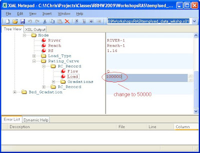
In the sediment data, rating curve boundary condition editor, there is a bug in "saving" the total load. The first time you enter it, everything is fine-works great. However, if you change anything in the rating curve editor, save it, close the sediment data editor and then reopen it, you'll see that the original data is back in. RAS won't save new edits to the rating curve window in the current version (version 4.0). An easy way to get around this is to save RAS, close RAS completely, then open up the *.s01 (or *.s02, *.s03, whatever sediment file you are using) in a text editor. If you have an XML editor, it will be easier to sift through the data and find what you want to change. Then, find the data you wish to change and manually change it in the editor, external to HEC-RAS. Then reopen HEC-RAS, and you'll see the changes have been made. Caution! Be careful when making edits in the text editor. If you accidentally change any of the syntax, you could corrupt the sediment file, making it partially or totally unreadable by HEC-RAS. To be safe, it's not a bad idea to make a backup copy of the original file, before you make any edits to it.

Make changes in a text editor

or make changes in an XML Editor (easier)

Tuesday, March 3, 2009

Caution with interpolating cross sections

Written by Chris Goodell, P.E., D. WRE | WEST Consultants
Copyright © RASModel.com. 2009. All rights reserved.

The interpolation feature in HEC-RAS makes it very easy to add cross sections to satisfy numerical spacing requirements. Althought the routines are very robust and easy to use, caution should be used when interpolating between cross sections with multiple blocked ineffective flow areas. While normal ineffective flow areas are interpolated quite well (provided there are ineffective flow triggers on both bounding cross sections), multiple blocked ineffective flow areas are NOT interpolated.

So if you have multiple blocked ineffective flow areas on either of the bounding cross sections, you must manually add the multiple blocked ineffective flow areas to the interpolated cross sections. I suggest using the graphical cross section editor when doing this, especially if you have a lot of cross sections to fix.

Thursday, February 26, 2009

Minimum Flow requirements

Written by Chris Goodell, P.E., D. WRE | WEST Consultants
Copyright © RASModel.com. 2009. All rights reserved.

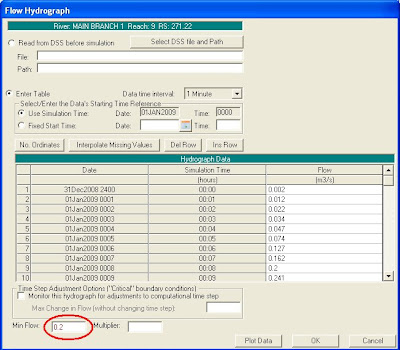
It's common knowlege that HEC-RAS cannot go "dry" at any time during a simulation. However, very low depths can be problematic as well. Very low depths can lead to compounding errors that can cause instabilities, and eventually your model to crash. There are a couple of tricks to get around this problem. Pilot channels and added base flow. None of you inflow hydrographs should start with 0 inflow, unless there is sufficient backwater in you system to prevent the upstream cross section from going dry. The trick with adding base flow is to keep it as small as possible, while providing the necessary stability. Try 1% of the peak of the hydrograph. You definately do not want to add a significant amount of volume to your model before the flood wave arrives-that will limit the extent of hydrograph attenuation you'll get.

To add base flow to an inflow hydrograph, simply add a minimum flow value in the box at the lower left corner of the flow hydrograph editor. Then, for that hydrograph, RAS will use the base flow amount any time the hydrograph flow is less than the minimum flow value.

Wednesday, February 25, 2009

HEC-RAS Short Course-Basic and Sediment Transport!

Next month I will be teaming with Gary Wolff to teach an HEC-RAS short course through River Restoration Northwest. The course will be in Tacoma, Washington, March 23-27. Gary will be teaching Basic RAS the first 3 days, and I'll be teching Sediment Transport with RAS that last 2 days. If you're interested, don't wait too long, last year we completely booked up the same course. You can get more information and register at http://www.rrnw.org/index.html.

Tuesday, February 24, 2009

Wide Flat Cross Section Bottoms

Written by Chris Goodell, P.E., D. WRE | WEST Consultants
Copyright © RASModel.com. 2009. All rights reserved.

A common problem with the import of cross sections from GIS that were developed with a terrain model generated from LIDAR is the cross section with a flat bottom. This is a result of LIDAR's inability to penetrate the water surface. As a result, you get a flat bottom that represents the water surface elevation in the channel at the time the LIDAR was taken.

This will cause problems right from the beginning of your simulation, particularly if you are running low flows (low depths), and your model will most likely crash right away. You can see the result of the lack of bathymetric data in the profile plot.
To fix this, you'll need to get some definition to the bottom of your cross section(s), either by approximating the channel bottom, or by field surveys.

Saturday, February 21, 2009

n Values in Graphical XS Editor

Written by Chris Goodell, P.E., D. WRE | WEST Consultants
Copyright © RASModel.com. 2009. All rights reserved.

Until the new version 4.0 came out, the most you could do with n-values in the Graphical Cross Section Editor, was to move around their respective breakpoints. Now you are able to directly change the n value in the Graphical XS Editor. You do this by simply clicking on the n value on the plot. You'll see it change to an input box that allows you to edit it. When done, just click away from the box and your new n value is entered. Make sure you advance to the next cross section so that the change is saved to memory.

Thursday, February 19, 2009

Severe Energy jump at junctions for unsteady flow

Written by Chris Goodell, P.E., D. WRE | WEST Consultants
Copyright © RASModel.com. 2009. All rights reserved.

A limitation in HEC-RAS unsteady flow is that at junctions, RAS will project the downstream water surface elevation to the 2 upstream cross sections across the junction. Then the energy grade at each upstream cross section is back calculated. The result, especially if your cross sections are spaced far away from the junction is a depth that is too low at the upper cross sections, resulting in a large velocity head, and a huge jump in energy. To balance the energy from that cross section to the next one upstream results in a large increase in water surface elevation. This is a common experience at junctions in unsteady flow modeling and will look similar to this in a profile view. A tell tale sign of this problem is if you see the cross section on the upstream side of the junction go supercritical.


The way to fix this is to move your cross sections as close to the junction as possible (or add cross sections closer). This will minimize the negative affect of the junction limitation in RAS. Also, adding more cross sections between the cross section just upstream of the junction, and the next one upstream, will minimize any residual jump in water surface elevation while trying to balance the energy.

Thursday, February 12, 2009

Breach Progression-Linear or Sine Wave?


Written by Chris Goodell, P.E., D. WRE | WEST Consultants
Copyright © RASModel.com. 2009. All rights reserved.

I get this question a lot. Do I use a linear or sine wave dam breach progression? The concept of the sine wave breach progression is that the breach will initially grow at a slow rate (when the breach just begins to form, not a lot of head on the breach), then it will speed up as velocities and shear stress picks up through the breach. Then it will slow down again at the end of the breach as the water level in the reservoir reduces to a small amount over the breach invert.
There's no real research out there that I know of that addresses this. The way I look at it is if my reservoir draws down with my breach (slow breach/small reservoir case), then the sine wave progression makes more sense to me. If my reservoir remains high as the breach is forming (fast breach/large reservoir case), then the linear progression makes more sense to me (actually a combination of the two makes the most sense to me in this case-this can be done by manually chaning the values in the table on the side to start out as a sine wave and then transform into linear). In all honesty, I usually incorporate the breach progression into my sensitivity analysis, and eventually go with the more conservative of the two.


Wednesday, February 11, 2009

How to best model a junction.

Written by Chris Goodell, P.E., D. WRE
Copyright © RASModel.com. 2009. All rights reserved.

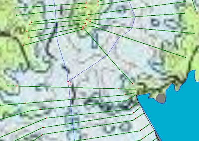
Here is an example of a junction.
With junctions, generally it is important to get cross sections as close to the junction as possible-even more so with unsteady flow modeling (http://hecrasmodel.blogspot.com/2008/12/unsteady-flow-and-junctions.html).

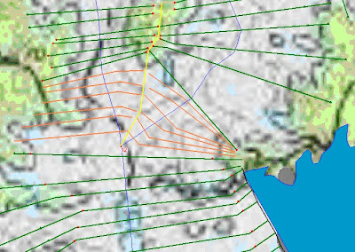
With this example, I would certainly add more cross sections upstream of the junction like so…


What I’ll usually do is draw an approximate “plane of confluence” (the yellow line), and then butt the new cross sections up to that line, without crossing over it. This plane of confluence will generally follow high ground between the two reaches, but technically should define the boundary between flow lines of one reach and flow lines of the other reach. The new cross sections will be missing the high ground on its “confluence” side, but that’s okay, because the other cross section (in the opposite reach) will capture that.

You certainly do not want cross sections overlapping or extending into another reach’s flow path. Sometimes you’ll find that interpolated cross sections might overlap at times. That’s okay as long as it is just a geometric schematic issue, and that cross sections were not really surveyed overlapped.


Thursday, February 5, 2009

Crazy Energy Grade Line

Written by Chris Goodell, P.E., D. WRE | WEST Consultants
Copyright © RASModel.com. 2009. All rights reserved.

Sometimes you may find in your unsteady flow simulation a nice smooth water surface profile, but then you turn on the energy grade line and it looks terrible. For example, in this steep section, the energy grade line is obviously incorrect. More times than not, this can be fixed very easily by adjusting the htab parameters. Sometimes in HEC-RAS, the HTAB parameter "starting elevation" is set too high by default. If you have a very low water surface elevation (i.e., well below the first HTAB computation point as shown in the figure), then HEC-RAS has a difficult time computing the energy grade line. This can create errors that may lead to instabilities. By changing the starting elevation for HTAB development to the invert elevation of the respective channel (and maybe providing more resolution by adjusting the increments and number of points), you can smooth out the energy grade line.


Thursday, January 22, 2009

Theta Implicit Weighting Factor

Written by Chris Goodell, P.E., D. WRE | WEST Consultants
Copyright © RASModel.com. 2009. All rights reserved.

The Theta Implicit Weighting Factor is used in unsteady flow HEC-RAS as a means for providing numerical stability through the imiplicit solution of the St. Venant Equations. Without going into the details, a value of 1 for Theta provides the most stability, but sacrifices some accuracy. A value of 0.6 provides the most accuracy, but is very difficult to stabilize. So...what should we use for our unsteady flow models. There is some disagreement out there among users of HEC-RAS, but here is my take: The manual, and the class that HEC holds suggests working with a Theta value of 1.0, then when your model is stabilized, reduce it as close to 0.6 as possible. In my experience, moderate to complex models never are able to maintain stability with Theta less than around 0.8. At some point in the past, I realized that most of the time, reducing the Theta value did not produce significantly different results. However, many modelers insist that Theta should be reduced. I can't disagree with that. In principle, I believe this is correct. However, in practice, my experience shows that it makes very little difference.

I think this would make a great topic for a paper, and the research would be easy to conduct. Does anyone have any thoughts on this topic?

Thursday, January 8, 2009

Where will my dam breach flood go?

Written by Chris Goodell, P.E., D. WRE | WEST Consultants
Copyright © RASModel.com. 2009. All rights reserved.

One of the first steps (usually in the proposal stage) of a dam breach model is to visualize where the flood wave will travel downstream from the dam. Is there a very obvious main channel entrenched in a canyon (if so, you have a fairly easy task). Many times, dam breach models are not this straight-forward. I have this dam breach project I'm getting ready to start. Just below the dam, two tributaries (fairly canyonized) converge with the primary stream. This spot is wide open and flat. My dilemma is how do I set up my model just below the dam. Water will come out of this breach and go up both tribs and probably swirl around quite a bit just downstream of the dam before eventually heading down the primary stream. Originally I thought about coupling a 2-D model with RAS, but that can be a real pain (not to mention possibly blow the budget). I'm now thinking of setting up the downstream area as a Storage Area in RAS with both secondary tribs included as part of that storage area. Then I'll connect the primary reach to the storage area so that the dam breach flood wave can drain downstream. I've placed inline storage areas further downstream in dam breach models, but never just below the dam. Hope it works. I would love to hear any comments or suggestions...