This is a great presentation put together by Mr. Steven Piper of the Hydrologic Engineering Center that discusses in detail the use of “Rules” at inline structures. Dr. Michael Gee forwarded this presentation to me after seeing some discussion on the forum about the use of Rules for inline structures. Thanks for the suggestion Dr. Gee! Mr. Piper kindly provided permission for me to post this to RASModel.com. This presentation is also available to download at:
https://drive.google.com/file/d/0B0bpiyLiUeRXNnVLMnNDNGVnWkE/view?usp=sharing
Enjoy! 
The advanced rules allow sophisticated control of hydraulic structures (inline structures, lateral structures, storage area connectors, and, in the next RAS version, pumps).
This presentation is only an overview. To get a working knowledge of the rule capability in RAS, it is recommended that the user read the detailed documentation in the User’s Manual.

The operating procedures for determining and controlling the releases from reservoirs and other types of hydraulic structures can be quite complex. HEC-RAS allows flexibility in modeling and controlling the operations of hydraulic structures through the use of rules. The rules can be used to operate the height of the gate openings. Alternately, the rules can directly control (or constrain) the flow despite the gate openings (or even without gates at all). Examples of variables that could be used to control releases from a hydraulic structure are: current flows and water surfaces at the structure, current flows and stages at downstream or upstream cross section locations, time considerations (winter, morning, etc), and/or previously computed values (accumulated outflows, running averages, etc). Rule operations in HEC-RAS are available for inline hydraulic structures, lateral hydraulic structures, and storage area connections.
Rules for controlling hydraulic structures can be entered after an inline structure, lateral structure, or storage area connection has been added to the project. From the Unsteady Flow Data editor, add or select the given structure and then click on the Rules button. This will bring up the Gate Rule Operation editor (as shown in the next slide). In the Gate Parameters table at the top of the editor, some initial information can be entered for any gate groups that are in the hydraulic structure.
The Open and Close Rate controls how fast the gates can move. So if, for example, a rule operation required the gate to open one additional foot and the gate opening rate was 0.1 ft/min and the user had selected a one minute time step, it would take ten time steps for the gate to reach the new opening height.

The Open and/or Close Rate can be left blank, which means the gate can move to any new setting in a single time step.
The Max and Min Opening will constrain the maximum and minimum gate opening settings. Building on the previous example of opening the gate one additional foot, if the gate was at 3.5 feet and the maximum was set to 4 feet (even though the gate was 6 feet tall), over a five minute period, the gate would open to 4 feet and then stop. If the Max is left blank, then the gate maximum opening is limited only by the height of the gate. If the Min is left blank, then the minimum opening is fully closed (i.e. 0.0).
The Initial Opening provides the first setting for the gate. This opening height will be used during the initial backwater computation. The gate will be left at this setting until it is changed by a rule operation. The Initial Opening is required for all gate groups, if any, in the hydraulic structure and may not be left blank.
In this example, row 7 is getting the wsel at the dam. Row 13 is checking to see if it is 0600 hours. If it is, then rows 17 and 22 are executed. Row 17 computes a new gate opening elevation for the drop gates. The new elevation is 3.5 feet below the wsel at the dam. Row 22 converts the elevation into an actual gate opening and tells the program to use the new gate opening. The final result is that at 0600 hours the drop gates are adjusted to have 3.5 feet of head on them.
To enter or edit the rule operations, click the Enter/Edit Rule Operations button.

 Operation Types
:
Comment. Provides a user entered line of text (for documentation only).
New Variable. Allows the user to create a variable and give it a custom name.
Get Simulation Value. A variable is set equal to a given value in the simulation, such as the flow at a cross section or the time of day.
Set Operation Parameter. Changes the operation of the hydraulic structure, for example, adjusting the gate height or setting a maximum discharge.
Branch (If/Else). Controls which operations are executed on the basis of an If-Then test (e.g., do different gate operation checks based on seasonal considerations).
Math. Performs math operations such as summing flows or averaging water surfaces.
Table. This operation allows the user to enter a table and perform table lookups to get a value.


A group of rules for one hydraulic structure is referred to as a rule set. At the start of each time step, each rule set is evaluated to check for changes to the operation of the given hydraulic structure. Rule operations are performed from the first (top) rule to the last (bottom) rule. By default, each rule operation is evaluated once. However, branching operations (If/Then/Else, etc) can cause some rule operations to be skipped. No looping or jumping to prior rule operations is allowed. That is (during a given time step), a rule operation may not be performed more than once.
Note: A rule set is only called once during a time step, even if the program iterates during that given time step. (Whatever rules are “in force” at the start of the time step will apply during all of the iterations).
The Get Simulation Value operation provides information about the current state of the model.
In the above example, the wsel at a cross section just upstream of the dam is being retrieved and stored in a variable named “WSEL at dam.”
There are currently seven categories of simulation variables. These are Time, Solution, Cross Section, Inline Structure, Lateral Structure, Storage Areas, and Storage Area Connectors. Clicking on the “+” will expand the list for that category.
For all the variables under Time, the user can select to use the time at the beginning of the time step (default), the end of the time step, or the previous time step.
For the remaining [non-time] variables, the user can select the current value, the value from the previous time, or a “look back” value.


Clicking the
Math operation button creates a math operation as shown. The result of the math operation can be assigned to either a new variable or an existing variable.
The math operation itself is composed of up to four different “expressions.” Each expression that is defined will return a real number. Expressions should be defined from left to right. So if a math operation is composed of two expressions, the left two expressions should be defined
and the right two expressions should be left as “[not set]” (i.e. they should be left blank). If more than one expression is defined, then the user must choose an algebraic connector from the drop down menu between them. The choices are: addition, subtraction, multiplication, and division.


In order to use a variable in an expression, or store the result into an existing variable, the user selects the variable with a pull down menu, as shown.
In row 129, there is a two part If/Then. In the first part, the rule operation is checking to see if “Canal Dam Vol since midnight” is greater than or equal to “Canal Dam Vol Diversion.” In the second part, it is checking to see if “Green Dam 4 Hour Ave Flow” is less than 10. Since the two different parts are connected with an “Or,” if either part is true, the expression will be true and rules 134, 135, and 136 will be executed. In more understandable terms, there is a check to see if the maximum amount of water has been diverted, or if the four hour running average flow at Green dam is below 10 cfs. If either is true, then all of the gates will be fully shut (and no more flow will be diverted for the rest of the day).

To control a given aspect of he hydraulic structure, a Set Operational Param rule operation is used. In the example above, rule 63 is setting the “gate flow desired” to the [previously calculated] value of “Flow New.” This will cause the RAS program to adjust the gate settings in order to get the desired flow. (The actual computed flow may be slightly different due to convergence tolerances and changing water surface elevations.)
There are a number of different operational parameters that can be set. In addition to setting the gate opening height or having RAS compute the height to get a desired flow, the user can: set a maximum flow, set a minimum flow, fix a given flow, etc.


In this simple example, a rule set that is attached to a lateral structure is being used to divert flow from the main river. The diversion is based both on the amount of flow going through a downstream dam and the time of day.
After getting the time of day and the flow at the inline structure, the actual diversion is determined from a lookup table as shown above. So, for instance, if the time is 12 (i.e. 1200) and the flow through the dam is 10,000 cfs, then 1000 cfs will be diverted.
In this example, the user has selected to interpolate. So if, for example, the flow was 11000 at
12 hours, then the flow diverted would be 1100 cfs. Instead, the user could have selected “nearest index value” which would have resulted in 1000 cfs being diverted for a main river flow of 11000. This option could be useful, for instance, if the lookup table was being used to set gate openings that can only be opened in discrete amounts.
Note that in row 13, the flow diversion (‘Flow to Divert’) has been set as a “Total Flow (Fixed)”. This means that the flow being diverted by this lateral structure is being entirely controlled by the rules (and the value from the lookup table). There are no gates and no hydraulic computations (e.g. computed flow over a weir).


In this, and following, slides, the gate control will be switched from elevation control to a rule set that has the same basic functionality.

The gate opening rates, maximum, minimum and initial gate opening are entered.
Next, the <Enter /Edit Rule Operation> button is clicked.


The first rule that is needed is the water surface elevation immediately upstream of the inline structure.
Clicking the <Get Sim Value> button, as shown, will start the creation of the first rule.


On the left, beneath where it says “Assign Result”, a descriptive variable name should be entered (in this case, WSEL).
Under Simulation Value, the Cross Section tab should be expanded and WS Elevation chosen.
Next, the river station just upstream of the inline structure is selected from the pull down menu.
On the right, the default “Value at current time step” should be left as-is. This gets the water
surface at the start of the timestep. Other choices would get a previous water surface or a
lookback/time-averaged water surface.


The next step is to add a rule that checks to see if the water surface is high enough that the gates need opening.
Clicking on the <Branch (If/Else)> button, will start the second rule. The If test compares the value of two different “Expressions”. Clicking on <Edit> underneath the Expression on the left will bring up the Edit Rule Expression editor as shown. Clicking on the Variable pull down menu will show all of the variables in the rule data set. In this case there is only one. Selecting the variable WSEL (which is created by rule 1), allows the value of the water surface to be compared to the second expression. Since the water surface is the desired item, the rest of the fields are left blank. (If it was desired, the Variable could be multiplied by a Coefficient, raised to an Exponent, and/or a Constant added.


For this If test, the check is to see if the water surface is greater than 6.0 feet. Between the two Expression buttons, there is a pull down menu that is used to select the “>” (greater than) operator.
The right Expression is clicked and the number 6 is entered in the Constant field.


The next rule is to set the gate opening height when the water surface is above 6.0 feet.
Clicking the <Set Operational Param> button will display the menu on the lower left and the
Gate.Opening operation is selected. Under Select Gate Group, the Left Group is selected.
The gate opening is set to 10.0 feet using the expression editor.


Every If rule must have a corresponding End If. Click the <Branch> button, which initially creates an If rule. Change this rule to an End If by the selecting the End If radial button as shown.

Another conditional must be created to close the gates when the water surface gets low enough.
The quickest and easiest way to do this is by making a copy of the existing rules (that open the gates), and then editing the copy.
Highlight rules 2 through 4 by clicking on rule 2 and then pressing the down arrow while holding the shift key (shift + down arrow).
Next, click on the Copy button, then move the cursor below row 4 (as if a new rule was to be made using one of the standard Insert New Operation) and then click on the Paste button.
The keyboard shortcuts Ct+X and Ctrl+V, can be used instead of clicking on the copy and paste keys.
Copying existing rules using the Ctrl+X and Ctrl+V shortcuts (and then editing the copy) can save a lot of time and effort.

The next step is to edit the just copied rules.
The 6 needs to be changed to a 4 (in the If rule), the operand needs to be changed from a greater than to a lesser than, and the gate opening value needs to be changed from 10 to 2.


Finally, it is a good idea to click on the <Check Rule Set> button. RAS will check for any basic errors in the rule data set. (For instance, if there is a If rule that does not have a corresponding End If.) If the Check Rule is not performed at this stage, RAS will still perform the check at run time. Errors will generate a message for the user about the problem. The Check Rule button is
a short cut that allows the user to identify problems while the Operation Rule editor is still open.


In addition to If/Then, the rules also allow for If/Then/Else and If/Then/ElseIf/Else type constructions (as well as nested If/Then statements).
In the above example, the gate opening will be set to 10 if the WSEL is greater than 6.0 feet. Otherwise, the opening will be set to 6 feet if the WSEL is above 5.0 feet. Finally, it will be set to 2 feet if the WSEL is less than 4.0 feet.
If the WSEL is less than or equal to 5 feet, but greater than or equal to 4 feet, the gate opening will not be changed.


Deciphering (aka debugging) what a complicated rule set is actually doing can be tricky. RAS has a text based output file referred to as the Detailed Log. The operation of each rule in a rule set can be examined on a timestep by timestep basis from this log.
The log output is turned on as shown above.


Every rule that is executed will be shown—as will the result of that rule. The output shown above is taken from the previous rule data set that opens the gate when the WSEL is greater than
6.0 feet.
Rule 1 is executed and the variable WSEL is set to the water surface which is around 6.01 feet. Rule 2 is executed and this rule is True because the value of the first expression (~6.01) is
greater than the second expression (6.0). Rule 3 is executed and the gate opening for the Left Group is set to 10 feet. No other rules are executed for this rule data set (for this time step). Use the find function to locate when things happen. For instance, the string “0002 True” was searched on to find this location in the log file.
Note: having detailed (debug level) output for the rule data set directly available within the
GUI is already on the RAS “wish list”.


The canal data set (which is included as one of the sample data sets when RAS is installed) provides a good example of the sophisticated operations that are possible with the advanced rule capability.
In this data set, the rules are being used to allow RAS to model a reservoir and a water supply canal in Florida. The Florida water district has a complicated operating agreement that it must conform with.
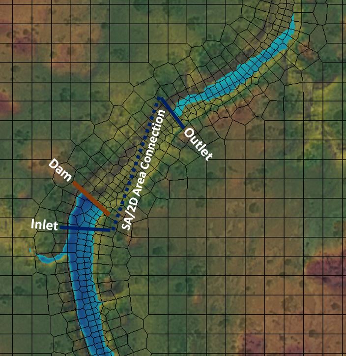
A reservoir has been modeled as a series of cross sections. A water supply canal leaves the side of the reservoir. This has been modeled with a junction and an inline structure (shown above and red circle) on the diversion canal. The main dam on the reservoir is further downstream (and is not shown on the above graphic).
The flat terrain (river gages suffer backwater effects far upstream of the dam) and the large groundwater flows make measuring inflows to the reservoir difficult. Instead, the inflow to the reservoir is assumed to be equal to the outflow (the outflow from the main dam plus the outflow through the water diversion canal).
The water district’s allowable diversion is based on the previous day’s outflow (midnight to midnight). Additionally, the water district is not allowed to divert water when the outflow from the main dam is too low. (The flow at the main dam is reduced when the reservoir drops too low—so, the water district is, indirectly, prevented from making diversions when the reservoir water surface is low.)


Rules 3 through 5 create three variables. New variables are most often created with a Math or Get Sim Value operation. However, it is sometimes convinent to have the variable creation be its own rule. Note: the Initial Value = 0 sets the variable equal to 0.0 at the very start of the simulation (the very first time the rule set is called for the first timestep). Afterwards, the variable will keep its value between time steps (e.g., if it equal “5” at the end of the first time the rules set is called, it will equal “5” at the start of the next time). To set it equal to 0.0 at the start of each time step, a Math operation should be used.
Rule 10 gets the length of the time step with a Get Simulation rule. A math operation is then used to compute the length of the time step in seconds.
Rules 16 and 17 get the outflow from the main dam and the diversion canal.
Rules 20 and 21 add the volume of outflow (for this time step) to the current volume. The
“current volume” is the volume of outflow since midnight.
Rules 26 and 27 get the day of the month at the beginning of the time step and the end of the timestep. If the data set is using 15 minute time steps, at some point the beginning of the timestep will be at 11:45pm and the end of the timestep will be at 12:00am. When that happens, the beginning day of month will not equal the end. Beginning might be 5 and ending 6, or beginning could be 31 (or 30 or 28) and the end will be 1 (the first of next month).
Note: The rules use a 24 hour clock, so in the above example, the timestep would actually be at
23:45 and 00:00.


Rule 31 checks to see if it is midnight. When the timestep starts and ends on different days, it is midnight.
Rule 39 computes the total average outflow for the previous 24 hours (in cfs). Rules 42 and 43 zero out the volume variables for use for the next day.
The methodology for determining the allowable diversion is based on the amount of outflow. No diversion when the flow is less than 100 cfs (rule 47). 10% of the previous days flow when the flow is between 100 and 150. A sliding scale (from 10% to 30%) when the flow is between
150 and 215. 30% for flows between 215 and 1000 and a maximum of 300 cfs (for flows over
1000).


Up to four separate expressions can be combined into a single Math operation.


Rule 69 converts the allowable diversion from cfs to a daily volume.
The gates are adjusted at midnight and are left in place until the allowable diversion has taken place. The gate flows are computed so that the diversion will take approximately 20 hours. (If the flow was based on a 24 hour diversion and the gate flow was slightly less than assumed, then the gates would either have to be adjusted or the full, allowable diversion would not take place).
Rule 77 computes the 20 hour flow on a MGD basis.


The inline structure has three different gate groups (that are used in normal operations). The gates are overflow (drop) gates.
For each gate group, the water district has a table that shows the amount of head that should be on that gate group for a given flow.
Rule 80 computes the amount of head needed on gate group #1 using the lookup table (shown above). The value that goes into the lookup table (input) is determined by the expression editor. In this case it is the “Canal Dam 20 hour MGD” variable (which the first part of the name can just be seen left of the lookup table). The result of the lookup (output) is stored in a new variable, “Head Opening #1”.


The head on the drop gate is the upstream water surface minus the gate opening height minus
the invert elevation of the gate. Rearranging, gives the gate opening to be equal to the head plus the invert minus the upstream water surface as computed in rule 100.
Rule 100 computes the desired gate opening.
Rule 105 actually sets the gate opening to the value that was computed by rule 100.
The computation for the gate opening involves two different variables (Head and WSEL), which meant that two different “Expressions” had to be used. The Set Gate Opening command only has a one Expression. So a Math operation was used (which can have up to 4 different variables/expression) in rule 100.


There are two different triggers for shutting the gates:
One trigger is the first part of rule 129. It checks to see if the allowable volume of water has been diverted. If it has, then rules 134-136 make sure all the gates are closed.
The other trigger is based on the outflow from Green dam. When the flow at Green dam is below 10 cfs, the water district must stop diverting water. (This only happens at low reservoir levels.) However, it is possible for the reported flow at Green dam to briefly drop below 10 cfs, either because of a switch in gate operations or because of a “missing value” from the remote data operation. To accommodate this, the water district does not have to stop the diversion until the average flow over 4 hours has dropped below 10 cfs.
Rule 124 computes a running, 4 hour average of the flow from Green dam. Looking at the lower right of the above screen shot, the Lookback period is from 4 hours ago to the current times step (0 hours ago).
The second part of rule 129 checks if this 4 hour average is below 10 cfs. If it is, all of the gates are closed.


The rules between an If/Then and it corresponding End If can be collapsed and/or expanded. This is done by clicking on the “+/-” to the left of the row number. This option can make viewing complicated data sets easier. (The rules are still active.) All of the rules that are involved in the once daily computations (at midnight) have been collapsed, above.

 But we're in luck! Mr. Con Katsoulas, a senior water resources engineering from SMEC in Sydney Australia came up with a method to get around this limitation. He first discussed this in The RAS Solution forum. And my friend and colleague, Mr. Krey Price of Surface Water Solutions wrote a detailed explanation on how to use this technique. Please read his blog post on wormhole culverts for the full description.


