Cross Section Points Filter

Written by Chris Goodell, P.E., D. WRE | WEST Consultants
Copyright © RASModel.com. 2010. All rights reserved.
Now that a lot of us use GIS to generate our cross sections, this is becoming a much more “used” feature in RAS: The Cross Section Points Filter. RAS allows a maximum of 500 station-elevation points in any given cross section. It is very common for one or more cross sections cut in GIS to come in with a LOT of station elevation points. And then, if you interpolate cross sections (interpolated cross sections have more-or-less double the station elevation points as their bounding sections) you’ll have even more points. Exceeding 500 points in a cross section is very easy to do.

RAS offers a few ways to filter out points. There is the “Near and Co-linear” filter. This allows you to specify a tolerance for points that are very close to each other, and points that are in a straight, or nearly straight line. RAS will then remove points that are within the tolerance level (i.e., if you have three points in a perfectly straight line, there is no need to include the middle point in your geometry-unless it happens to be a bank station or n-value break point, in which case RAS will preserve it).

However, my preference normally is to use the “Minimum Area Change” option. RAS will remove points sequentially in an effort to minimize the area change of the cross section. You, as the user, simply specify the number of points you want RAS to filter to, and all the work is done for you. This is a much more convenient way to filter points-and much faster, but be aware that you have a lot less control over how the points are filtered. If you have a lot more than 500 points to begin with, it is a good idea to compare the “before” and “after” cross sections to make sure the new cross section preserves the true geometry. In my experience RAS does a great job at filtering using the Minimize Area Change option.

If RAS tells me there are a lot of cross sections that need to be filtered, I’ll use the “Multiple Locations” tab to get them all done at once. Select all the cross sections in your geometry (even the ones that don’t exceed 500 points) and RAS will only filter the cross sections that need filtering.

Contraction and Expansion Losses for Unsteady Flow

Written by Chris Goodell, P.E., D. WRE | WEST Consultants
Copyright © RASModel.com. 2010. All rights reserved.
Since unsteady flow was introduced in HEC-RAS years ago, the contraction and expansion loss coefficients were not used, because losses due to contraction and expansion were automatically approximated in the conservation of momentum equation. Since steady flow RAS does not use the momentum equation for backwater computations, we had to approximate the contraction and expansion losses using those loss coefficients that you see for every cross section in the cross section editor. When switching to unsteady flow, you could leave those coefficients in every cross section; RAS just won’t use them.



In the latest version of RAS (version 4.1), the release notes indicate that RAS may not be capturing all of the C&E losses in unsteady flow, particularly at sharp contractions and expansion. And therefore, unsteady contraction and expansion loss coefficients can now be used.

From the 4.1 Release notes:, “In general, contraction and expansion losses are not used in unsteady flow, and therefore the default coefficients are 0.0. Forces due to contractions and expansions are handled in the momentum equation through pressure force differences. However, because HEC-RAS is a one-dimensional unsteady flow model, the one-dimensional momentum equation does not always capture all of the forces action on the flow field at a sharp contraction and/or expansion zone. In order to better approximate the forces acting on the water, and the resulting water surface elevation, at a contraction and/or expansion, the user can enter empirical contraction and expansion coefficients for unsteady flow modeling. These coefficients will be multiplied by a change in velocity head, just like in steady flow modeling, but the resulting energy loss gets converted to an equivalent force for placement into the momentum equation.”

Notice that there is a new table for entering unsteady flow contraction and expansion losses.



So the obvious question is, “what values do we use for unsteady flow contraction and expansion coefficients?” Are they the same as their steady flow counterparts? Also, when do we want to use them?

Any suggestions out there???

Probabilistic Methods for Dam Breach Modeling

Written by Chris Goodell, P.E., D. WRE | WEST Consultants
Copyright © RASModel.com. 2010. All rights reserved.
I would appreciate any feedback from you all on this topic. It's something I've been thinking about for a while now. My biggest concern with the current practice of dam breach modeling is the overwhelming uncertainty associated with dam breach parameters. Not only the ultimate breach shape and development time, but things like the initiation mechanism of the breach, the discharge coefficients (both weir and orifice), and the progression rate. The deterministic approach we use leaves a bit to be desired in my opinion. Sensitivity analyses have shown that the breach outflow hydrograph can easily vary by 100% or more, based on the set of parameters used. I've been considering ways to generate a breach outflow hydrograph based on probabilistic methods. The idea being instead of providing our "best conservative guess" for the breach hydrograph, we can produce a 95% (or whatever percent) conditional non-exceedance hydrograph based on both overall peak discharge and also timing. Meaning, this is the dam breach hydrograph that will not be exceeded in peak value 95% of the time, given a dam failure for a given failure mechanism (overtopping or piping). This is done by assigning probablity distribution functions to each breach parameter, then run a Monte Carlo simulation using random assignments (within the minimum and maximum bounds and following the prescribed distribution function) for each breach parameter. Then we can plug the resulting 95% hydrograph (or the associated set of breach parameters to create that hydrograph) into our HEC-RAS unsteady flow model and resume our deterministic approach. At least we have taken the deterministic selection of breach parameters out of the analysis. I suppose at some time, the entire model could be approached with probabilistic methods, but first things first. In fact, HEC is currently working on implementing Monte Carlo simulation capabilities into HEC-RAS for a future release.

I wonder if any state Dam Safety office is ready for this type of analysis for preparing inundation maps for emergency action plans. I think it makes more sense.

Dynamic versus Level Pool Reservoir Drawdown for Dam Breach Modeling

Written by Chris Goodell, P.E., D. WRE | WEST Consultants
Copyright © RASModel.com. 2010. All rights reserved.
This is a summary from a paper (Goodell,Christopher;Wahlin, Brian. “Dynamic and Level Pool Reservoir Drawdown: A Practical Comparison for Dam Breach Modeling.” 33rd IAHR Congress Proceedings, Vancouver Canada, 2009) on level pool versus dynamic reservoir drawdown for dam breach modeling. In RAS you can define your reservoir with a series of cross sections (which uses dynamic routing) or a storage area (which uses level pool routing). Dynamic routing is generally assumed to be more accurate, but the size and shape of a reservoir can sometimes make level pool reservoir adequate.

A key component to dam breach modeling is the reservoir drawdown. This has a significant impact on the magnitude and shape of the breach outflow hydrograph, and ultimately the extent of flood inundation in the downstream reach. Drawdown of the reservoir can be modeled with the precise and physically correct dynamic routing method, which uses the full St. Venant equations of Conservation of Mass and Conservation of Momentum. However, this requires detailed bathymetric data for the reservoir, which is frequently very difficult and expensive to obtain for existing reservoirs. Furthermore, dynamic routing is complex and prone to numeric instabilities. A level pool drawdown is a more simplistic, numerically stable approach that can be used successfully under certain circumstances and requires only a simple stage-storage curve for the reservoir.

Two primary characteristics emerge as indicators of a given reservoir’s ability to be described by a level pool analysis. The Compactness Factor, F_c, is simply the ratio of the dam height (H) to the reservoir length (L). The longer and shallower the reservoir, the lower the Compactness Factor and the more the reservoir acts like a river during its drawdown. Thus dynamic routing would be more appropriate in this situation. Short, relatively deep reservoirs are more compact, have a larger F_c value, and can be adequately described using a level pool analysis.

The Translation Factor, F_t, describes the relationship between the speed of the breach development and the ability of the reservoir to supply water to replace the water leaving through the breach. The easier the reservoir can deliver water to the breach, the more it can be described by a level pool analysis. Fast breach developments and long reservoirs are more appropriate to be modeled by dynamic routing. The Translation Factor is computed as:

F_t = ct/L

Where: c = shallow water wave celerity =.

d = representative reservoir depth.

and t = time.

A third parameter can be used to help graphically display the results of the various simulations. The Drawdown Number, D_n, is defined as the product of the Translation Factor and the Compactness Factor.






It becomes apparent that for high Drawdown Numbers, the level pool analysis produces results very close to dynamic routing. By enveloping the data points, a 5% threshold Drawdown Number is shown to be 0.41. That means that a reservoir with a Drawdown Number of 0.41 or greater will produce peak outflow results within 5% of a dynamic routing simulation. The 10% threshold Drawdown Number of 0.24 is also indicated on the plot.

You can see the full paper in the referenced proceedings. Also, the Hbox software has an automated utility for determining the appropriateness of level pool reservoir drawdown based on thd Drawdown Number analysis.

Dam Breach Modeling Q & A

Written by Chris Goodell, P.E., D. WRE | WEST Consultants
Copyright © RASModel.com. 2010. All rights reserved.
Some questions and answers related to dam breach modeling in HEC-RAS…

Question. The Sunny Day model has a consistent water surface elevation from the very start of the model – it only decreases once the breach occurs. How is HEC-RAS setting this starting WSEL?

Answer. You define the starting water surface elevation either by equalizing the flow from your outlet works with the reservoir inflow, or by setting an initial conditions water surface elevation in your flow editor and a pilot flow through the dam equal to the reservoir inflow at the beginning of the simulation.

Question. My breach models show a dramatic decrease in max Q from the cross-section immediately downstream of the dam to the end of the model. I know that HEC-RAS has an inherent storage routine that attenuates the flow throughout the model but is it reasonable to have a result that shows a beginning max Q of 12,370 cfs and an ending Q of 275 cfs (the reach is approx. 3.8 miles long with a slope of 0.02 ft/ft upstream and 0.001 ft/ft downstream)? This is an arroyo about 800-900 ft. wide, Manning’s at .055.

Answer. I would be skeptical of those results. Perhaps there is an error somewhere in the simulation, or you have a lot of flow leaving the system. Sometimes, if your model is not properly constructed, you can develop a large “wall of water” in profile view. A lot of times this is due to poorly defined HTAB parameters. This will create an artificial pool of water behind the wall, which will drastically attenuate your flood wave. Look in the profile plot and animate through your simulation. If you see an unexplainable wall of water backing up flow, that would be the cause.

Question. My models are stable but still have inherent errors (max iterations) and critical depth defaults to varying degrees. Does this have a significant effect on the model results? Changing parameters at this point to reduce inherent errors most likely will cause instability.

Answer. Max iterations are not necessarily a problem as long as the associated errors are small and it is not causing visible instabilities or obvious errors in your results. I try to get rid of all max iterations where possible. If not possible, I try to get the errors below 0.1 ft as much as I can (my own rule of thumb). RAS does not typically default to critical depth in unsteady flow (like it does in steady flow). But it sounds like you have areas that have flow close to critical depth. This can cause instability problems. If you believe flow should be close to critical depth in these locations, try turning on the Mixed Flow option and adjusting your LPI factor. If you do not believe flow should be near critical in these locations (most of the time in natural streams you should not see critical or supercritical flow), then you may be underestimating your Manning’s n values. Manning’s n values for the front end of dam breach flood waves and steep reaches are frequently underestimated. Check Jarrett’s equation if in a steep reach. Your reach slope of 2% is quite high. An n value of 0.055 is possibly too low during the low flow period preceding the dam breach flood.

Question. Does the number of vertices defining a cross section matter, in another words, does the model run better with cross sections that have fewer vertices but still accurately define the section, vs. similar sections that have many redundant vertices?


Answer. Better definition is usually advantageous. RAS does not like to have long horizontal portions of cross sections which is common for coarsely-defined cross sections. It can cause numerical problems. These days, having the maximum number of points in a cross section (500) typically does not noticeably slow down computation speed. I recommend getting as much detail as you can in your cross sections.

Bridge on a Spillway

Written by Chris Goodell, P.E., D. WRE | WEST Consultants
Copyright © RASModel.com. 2010. All rights reserved.
I just got an interesting question. How do I model a bridge that has a spillway just downstream of it? Here’s an example of what I’m talking about:



As I see it, there are a three ways to approach this. You could go conventional, and model both a bridge and an inline weir and try to squeeze in a couple of cross sections in between. This is probably the easiest, but not always possible if the bridge is on top of, or very close to the weir.

Another approach is to model the bridge as a bridge, and the weir with a series of closely spaced cross sections. This can be problematic if you have a high drop over the spillway with low tailwater elevations. And the cross sections will have to be very tightly spaced, to prevent over-estimation of energy loss over the weir. This is not recommended for vertical drop structures.

A third approach would be to model both the bridge and the weir together as an inline structure. The bridge opening can be simulated using a gate (or series of gates). The space between the gates simulates the piers. The gate invert is the top of the weir. The gate height then simulates the distance from the top of the weir to the bottom chord of the bridge. The upper chord of the bridge can be entered in as the top of dam. Make sure to leave the gate wide open for the entire simulation. Also, a nice advantage is that each gate can have it’s own weir discharge coefficient.



Any other suggestions out there?

Adding Help Files and References to RAS

Written by Chris Goodell, P.E., D. WRE | WEST Consultants
Copyright © RASModel.com. 2010. All rights reserved.
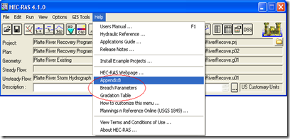
Everyone has their favorite references that they go to for help and guidance when developing hydraulic models. It could be the n-value table in Chow, or Tony Wahl’s Breach Parameter paper, or simply specific exerts in the RAS manuals. Whatever your preference, HEC has provided a very convenient way to easily access reference documents while in the HEC-RAS environment. You simply copy the document and paste it into the \Program Files\HEC-RAS\4.1.0 folder. You have to change the name so that the file begins with “RasHelp_”. That is how RAS recognizes it as a help document. Then when you open RAS, under the Help menu, you’ll see your custom documents listed for easy access. Notice that I have Appendix B of the RAS Hydraulic Reference Manual, a summary of Breach Parameter equations, and a Sediment Gradation Table in the Help menu.