Pages

Tuesday, December 24, 2013

Lateral Structure Coefficients

Written by Chris Goodell, P.E., D.WRE  |  WEST Consultants
Copyright © RASModel.com.  2013.  All rights reserved.
Lateral structures can be used in HEC-RAS to transfer flow from a river/reach to a storage area, or to another river/reach.  With the coming release of HEC-RAS with 2D capabilities (estimated beta release January/February 2014), you’ll be able to hook a river/reach to a 2-D area using a lateral structure. 
Although its primary function in HEC-RAS is to transfer flow out of one river/reach into another component (river/reach, storage area, 2D area), a lateral structure can physically represent a wide range of geometric features, including a levee, a flow diversion structure, a morning glory spillway, or even a natural ground or bathymetric profile.  Including a lateral structure in your model to represent a levee is important if the levee is ever overtopped or breached during the simulation.  Flow diversion structures can have multiple outlet features, including culverts, gates, and spillways.  These features are all available in the lateral structure editor in HEC-RAS. 
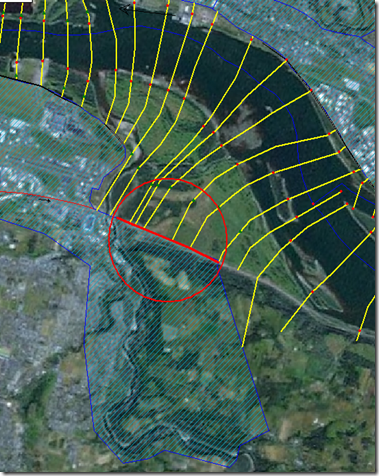
Another common use of lateral structures is to simulate flow transfer from the river to a tributary during a flood event.  This is especially convenient if you don’t want to model the tributary as an individual reach, but still want to account for it’s available storage, for a proper accounting of flood wave attenuation in the main stem river/reach.  As an example, the following figure shows a storage area representing a tributary to the main stem river.  This storage area is connected to the main stem by a lateral structure (highlighted in red). 
image
Because a lateral structure can represent a variety of different flow transferring structures (or non-structures), the hydraulics in and around the lateral structure can be quite different, depending upon the case.  Every lateral structure in HEC-RAS requires a lateral weir coefficient, and different hydraulics mean different lateral weir coefficients.  Any hydraulics textbook will have a multitude of weir coefficients for “inline” conditions, but it’s rare to find something similar for lateral flows, or diversion flows.  But it is generally agreed that lateral structure weir coefficients should be much lower than a similar inline configuration.  For example, an inline, hydraulically efficient broad-crested weir might have a weir coefficient around 3.0 (US units) or 1.7 (SI Units).  Turn that structure sideways (a lateral structure), and it will have a coefficient closer to 2.0 (US Units) or 1.1 (SI Units).  The difference is due to the energy/momentum loss associated with turning flow lines from their downstream orientation to a lateral direction out of the river/reach.    Unfortunately, there has simply not been a lot of research done on quantifying this energy/momentum loss and what that does to lateral weir coefficients.
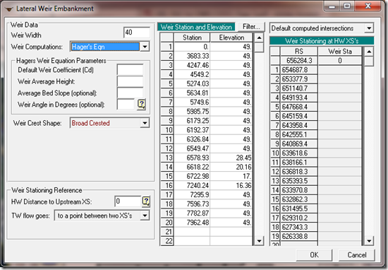
The research that is available could be useful and might be worth checking out.  Hagar’s equation is one reference and is actually built into the HEC-RAS lateral structure editor, under Lateral Weir Embankment…Weir Computations.  It will compute an equivalent lateral weir coefficient based on an inline value (the Default Weir Coefficient) and some physical and hydraulic properties of the weir and  the adjacent river/reach. 
image
You can read more about Hagar’s equation in the HEC-RAS Hydraulic Reference Manual on page 8-17. 
Useful references for lateral structure weir coefficients (including Hager’s):
  • Hager, W.H. (1987). “Lateral Outflow over Side Weirs.” Journal of Hydraulic Engineering, ASCE, 113(4).
  • Borghei, S.M.; Malili, M.R.; Ghodsian, M. (1999). “Discharge Coefficient for Sharp-Crested Side Weir in Subcritical Flow.” Journal of Hydraulic Engineering, ASCE, October, 1999.
  • Ranga Raju, K.G.; Prasad, B.; Gupta, S.K. (1979). “Side Weir in Rectangular Channel.” Journal of Hydraulic Engineering, ASCE, 105(5).
  • Subramanya, K.; Awasthy, S.C. (1972). “Spatially Varied Flow over Side Weirs.” J. Hydr. Div., ASCE, 98(1).
  • Singh, R.; Manivannan, D.; Satyanarayana T. (1994). “Discharge Coefficient of Rectangular Side Weirs.” Journal of Irrigation and Drainage Engineering, ASCE, 120(4).
However, none of these references discuss lateral weir coefficients for lateral flow transfers over natural ground, or surface flow (i.e. non-elevation overbank terrain).  HEC has a reference table for lateral structure coefficients that I like to use-it’s also included in the new “Combined 1D and 2D Modeling with HEC-RAS” document that was released in August 2013, in anticipation of the new 2D feature in HEC-RAS expected to be released as a beta version in the January/February 2014 time frame.   Note how low the suggested range of coefficients is for “non-elevated overbank terrain.”  Because they are not dimensionless, be aware that weir coefficients in SI Units are different from US units by a factor of the square root of the ratio of the SI gravitational constant to the US gravitational constant,
image

What is being modeled with the Lateral Structure Description Range of Weir Coefficients
Levee/Roadway – 3 ft (1 meter) or higher above natural ground Broad crested weir shape, flow over Levee/road acts like weir flow US Units: 1.5 to 2.2 (2.0 default)
SI Units:  0.83 to 1.2 (1.1 default)
Levee/Roadway – 1 to 3 ft (0.3 to 1.0 meter) elevated above ground Broad crested weir shape, flow over levee/road acts like weir flow, but becomes submerged easily. US Units:  1.0 to 2.0
SI Units:  0.55 to 1.1
Natural high ground barrier – 1 to 3 ft (0.3 to 1.0 meter) high. Does not really act like a weir, but must flow over high ground to get into 2D (or storage) area. US Units: 0.5 to 1.0
SI Units: 0.28 to 0.55
Non-elevated overbank terrain. Lateral Structure not elevated above ground Overland flow escaping the main river. US Units: 0.1 to 0.5
SI Units:  0.06 to 0.28

*Hydrologic Engineering Center, August 2013.  “Combined 1D and 2D Modeling with HEC-RAS”

Although this table is presented within the context of 1-D to 2-D flow transfers, these values will work with river/reach to storage area or river/reach to river/reach flow transfers as well.  As noted in the referenced document (HEC 2013), “In general, Lateral Structure weir coefficients should be lower than typical values used for inline weirs.  Additionally, when a lateral structure (i.e. weir equation) is being used to transfer flow from the river (1D region) to the floodplain (2D Flow Area), and then [sic] the weir coefficients that are used need to be very low, or too much flow will be transferred.”  Also, “The number 1 problem people have been having with interfacing 1D river reaches with 2D areas, is user’s [sic] have been using way to [sic] high of weir coefficients for the situation being modeled.  If the lateral structure is really just an overland flow interface between the 1D river and the 2D floodplain, then weir coefficients in the range of 0.1 to 0.5 must be used to get the right flow transfer and keep the model stable.” 

The HEC 2013 document ("Combined 1D and 2D Modeling with HEC-RAS") with the Table of lateral weir coefficients can be downloaded from my Google Drive site here:  https://drive.google.com/file/d/0B_s8OLJOgOi0Nm5sdHFhSzFUYkk/edit?usp=sharing.  The lateral weir coefficient table is on page 35.

Wednesday, November 6, 2013

Filtering Station Elevation Data in HEC-RAS

Written by Daniela Todesco | WEST Consultants
Copyright © RASModel.com. 2013.  All rights reserved.

I am working on a dam breach project where I’m trying to simplify a complicated model with dozens of tributaries and storage areas. In the process, I’m converting a few tributaries into storage areas (which are surrounded by other storage areas). For example, I want to convert the reach below (from 5.43 to 0.55) to a storage area. We happen to have the topographic data used to generate the original model (although we don’t have the original geodatabase), so we’re good to go. clip_image002 In order to do that, we need to delineate the storage area polygon, define new storage area connections, and generate lateral structures. The new “reach” (now a storage area) will look like the one below. clip_image003 Now we need station-elevation data for storage area connections and lateral structures. Easy, right? Well, not so fast. HEC-GeoRAS seems to have some issues exporting data when you take an existing project and try to modify shapefiles and extract data for only a portion of the entire model. It is especially difficult if you’re not the one who built the model in the first place. The shortcut is to think outside GeoRAS and obtain simple 3D station-elevation points directly from a TIN or grid for the storage area or structures you need. The bad part about that is that extracting tools in ArcGIS doesn’t really have an option to limit the number of points that are generated, and you end up with thousands of points that you can’t really use in HEC-RAS (the limit for cross section points, storage area connection weir/embankment points, and lateral structure weir points is 500). For example, in the connection called 83Coal in the figure above, I end up with over 2300 points. I’m stuck. Or so I thought… It turns out that RAS automatically “expands” its Station Elevation table to store however many points you need. In my case, 2339… image HEC-RAS will still give you an error if you try to run the model with this data (the limit of 500 points still stands for computations!), but a simple click of the “Filter” button you see in the figure above solves the problem. Voila! Hope you liked this new (for me) discovery.


Tuesday, October 8, 2013

Stabilizing a Dynamic Unsteady HEC-RAS Model

Written by Chris Goodell
Copyright © RASModel.com. 2013.  All rights reserved.

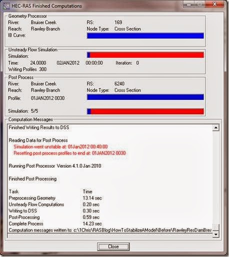
One of the most frustrating aspects of unsteady HEC-RAS modeling can be the model stabilization process. You know, you’ve gone to great lengths collecting the best survey/topo data and solid hydrology. Then you’ve painstakingly spent hours…possibly days entered all of that data only to find that once you press the “Compute” button, the model crashes. The dreaded “Red Bar”! clip_image002 Sometimes you can get your simulation to complete without crashing, but the listed numerical errors are so high that you can’t with good conscience submit that as your final simulation. Either way, approaching an unsteady HEC-RAS model (especially a dynamic one) as a beginner with little experience and understanding of how to stabilize it can cause significant delays in your project and worse, completely blow up your budget. I’ve uploaded two HEC-RAS projects to the following Google Drive Site: https://drive.google.com/folderview?id=0B_s8OLJOgOi0YU92SGZQZm9raWM&usp=sharing


RawleyResUnstable.prj is an unsteady flow dam breach HEC-RAS project recently sent to me for help. Although the model ran to completion without crashing, it had unacceptably high errors.
RawleyResStable.prj is the fully stabilized version of the model with no numerical errors.

The following lists out the courses of action taken to stabilize the model. Feel free to download the “Unstable” and “Stable” models and try these techniques on your own. The links following some of these items will take you to more information about that particular technique.
1. Cross Section Spacing. The initial spacing was way too coarse. A visual check alone of the geometry schematic and profile plot should encourage you to investigate a finer cross section spacing.
clip_image004
Geometry Schematic
clip_image006
Profile Plot Samuels equation suggests anywhere from 15 ft to 50 ft spacing (depending on what bed slope you use). I interpolated to 50 ft for the entire reach. http://hecrasmodel.blogspot.com/2008/12/samuels-equation-for-cross-section.html


clip_image008
clip_image010
  1. Dam Breach models typically have time steps on the order of a minute or less. This model was initially set with a computation interval of 10 minutes which is high even for the largest and “slowest” of dam breach models. I changed the time step to 10 seconds. The selection of 10 seconds was based on “gut” feel and lots of experience doing dam breach models. There are some methods for approximating good timesteps, notably the Courant Condition and Fread’s equation. Also, setting the cross section spacing/timestep ratio equal to a representative stream velocity will get you close. In this case, the cross section spacing is 50 ft, and I was able to pull some velocities (prior to the model crashing) at about 6 ft/s. That suggests a time step of 8.3 seconds. Close enough to 10 seconds, so we’ll stick with that.
  1. I changed the downstream boundary normal depth slope from 0.01 to 0.001. Not sure what is downstream of the first cross section, but 0.01 is awfully steep and was setting up a very low depth at the downstream boundary (which was causing instabilities). http://hecrasmodel.blogspot.com/2010/01/downstream-boundary-normal-depth.html
Notice in the following profile plot of the downstream end of the reach how the water surface at the boundary cross section is below critical depth (the red dot). This creates an overestimation of the water depth at the next upstream cross section, which in turns creates some instability over the next several timesteps.
clip_image012
The proper way to handle this would be to find out what is downstream of your model and select a boundary condition that best represents those conditions. In absence of downstream conditions, the 0.001 slope for normal depth provides a reasonable solution.  Either way, this underscores the importance of moving your downstream boundary far away from your area of interest in your study reach.  That way the errors that do originate from your downstream boundary assumption will have diminished to negligible levels before impacting your area of interest. 
clip_image014
  1. In the unsteady flow editor, the initial flow and the first time step flow should always be equal. In the original model, the initial flow is left blank (which is actually okay because RAS will use the first timestep flow if left blank). However, the first time step flow is very low at 0.14 cfs. Peak discharge of your inflow hydrograph is around 600 cfs. I put in a baseflow (minimum flow) of 5% of this, which is 30 cfs. Just to be safe, I put 30 cfs in the initial flow input box as well. It’s important to make sure that the 30 cfs baseflow does not have an impact on the peak of the breach outflow hydrograph. http://hecrasmodel.blogspot.com/2009/02/minimum-flow-requirements.html
  1. The upstream end of your reservoir is very steep (14%). This one was easy to spot in the profile plot because of the very nice smooth profile plot followed by a sudden spike in the energy level (green dashed line) at the upstream end. Notice to that there is a corresponding supercritical solution at the upstream most cross section. These are both indications that more cross sections are needed here. http://hecrasmodel.blogspot.com/2010/01/another-reason-for-interpolated-cross.html
clip_image016
I added more cross sections by interpolating the steep slope at the upstream end of the reservoir (10 ft spacing).
clip_image018
Notice the energy spike is not completely gone, but it is much better. Refining the HTAB parameters (http://hecrasmodel.blogspot.com/2009/02/crazy-energy-grade-line.html), turning on mixed flow and bumping up n values will collectively take care of the rest of this (see numbers 8, 9, and 10 below).
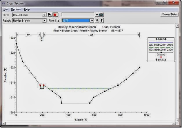
  1. From RS 4577 to 3791 you have your main channel defined in a small elevated side channel. The right overbank is lower in elevation than the channel.
clip_image020 This is problematic in RAS. Using the graphical cross section editor, I redefined the bank stations to get rid of this problem.

clip_image022
  1. Notice now in the HTAB parameters property table, the HTAB definition begins at the elevation of the invert of the side channel that was previously defined as the main channel. There is a big gap in the computation points in the newly defined main channel. This poses problems with HEC-RAS, particularly at low discharges/stages, since RAS will have to extrapolate to obtain a solution over that range.
clip_image024
I readjusted the cross section HTAB parameters to reflect the new bank station definitions (I used the “Copy Invert” button for all cross sections). While in there, I maximized the resolution of the HTAB parameters by changing number of points to 100 and minimizing the increment as much as possible while still having full coverage of each cross section. http://hecrasmodel.blogspot.com/2009/02/crazy-energy-grade-line.html http://hecrasmodel.blogspot.com/2011/03/more-on-htab-parameters.html
clip_image026
  1. In the figure below, notice all of the “red” areas in this zoomed in section of the  upstream end of the reach.
clip_image028
These are areas that are near critical depth. I turned on the “Mixed Flow” option in the Unsteady Flow Analysis window, which helps stabilize the near critical depths at the upstream end of the reservoir. http://hecrasmodel.blogspot.com/2011/04/mixed-flow-regime-options-lpi-method.html If you’ve been following along correcting your own copy of the model, you’ll notice that the model now finally runs to completion without crashing. There are still a few minor errors as shown in the Computation Messages.

clip_image029
It’s debatable whether you need to take care of these relatively small errors. Particularly for a dam breach model, where the presumed errors of the input data probably far outweigh these small numerical errors. Nevertheless, there’s a sense of pride in putting out a very robust model, completely free of numerical errors. So…let’s continue.
  1. The errors in the computation window above suggest a problem around river station 6200. That happens to be the upstream end of the reservoir and the source of the error can clearly be seen with the energy grade line and critical depth turned on.
clip_image031
The section at the upstream end of the reservoir is very steep at about 13.5%. In fact, that’s greater than the suggested maximum slope of 10%, as stated in the HEC-RAS manuals. You can see as the pool starts to lower, the steep reach is exposed and because of the low n values, the water surface is calculated to be supercritical. Let’s assume that the geometry is correct, and the upstream end of the reservoir really is that steep. Jarrett’s Equation suggests very high n values should be used here (~0.2), based on the bed slope and hydraulic radius (after the breach when the reservoir has drained). The original model had 0.07 and 0.035 for the overbanks and main channel, respectively. I changed all the n values in this steep reach to 0.15, because I think 0.2 might be a little overkill. http://hecrasmodel.blogspot.com/2009/12/n-values-in-steep-streams.html
There…no errors! However, there is still a Warning about extrapolating above/beyond the rating curve at a bridge (R.S. 277).
clip_image032
  1. To get rid of that warning, I increased the HTAB headwater maximum elevation at River Station 277 (the bridge) from 278 ft to 280 ft so that RAS doesn’t have to extrapolate.
clip_image033
There we have it. A clean solution. No errors, no warnings.
clip_image034


Thursday, October 3, 2013

Downstream Boundaries

Written by Chris Goodell | WEST Consultants
Copyright © RASModel.com. 2013.  All rights reserved.

I just received this question about downstream boundaries in HEC-RAS, and thought it would make a nice post here on RASModel.com.

"...regarding the boundary condition, if I use critical depth instead of normal depth will it be unacceptable?  When choosing the normal depth I need to enter a slope, can i use just one slope for the whole stream?"

Either critical or normal depth will work fine IF they are far enough downstream from your area of interest.  Normal depth is usually better, because it is typically a better representation of actual stream conditions.  Critical depth is only accurate when used at a significant grade break, a drop structure, a waterfall, etc., where flow passes through critical depth.  Critical depth does not happen in natural streams very often, and usually the water depth is nowhere near critical depth.  Using critical depth for a typical section of natural river is wrong.   That’s why I tend to always use normal depth.  However, using critical depth as a boundary condition is convenient (it’s easy to use, right?!?!), so it does have some merit. 

For normal depth, the slope you enter is not the slope of your modeled reach.  It represents the slope of the reach downstream of your downstream-most cross section.  You can often times approximate this slope by using a topographic map and locating where topo lines cross the stream, then measure the streamwise distance between them.  But remember this should be done DOWNSTREAM of your downstream cross section.  Normal depth as a boundary condition in RAS is applied to one cross section only-the downstream cross section, and using it means you are assuming that the reach just downstream of your downstream cross section is flowing under uniform (normal) conditions.  This too, is almost never the case in a natural stream due to the constant variation of cross section size and shape.  However, it is much closer to the true solution than critical depth is. 

The bottom line is both methods (in fact ALL methods) for assigning a downstream boundary have some inaccuracies.  That is why it is important to maintain distance between your downstream boundary and the area of your model that you are interested in.  One of the great things about the solution scheme in HEC-RAS is that it is "self-healing".  In other words, if there is an error at a specific location (due to a bad boundary condition, improper n value, poor survey data, that error will diminish the further away from that location you move.  At some point upstream, the effect of that error will no longer be "felt".  How far downstream you need to place the downstream boundary is variable, but you can test this by trying different downstream boundary assumptoins (critical depth and normal depth, or simply normal depth with a bunch of different normal slope assumptions) and seeing how far upstream you need to be to not see an effect from different downstream boundary assumptions.  This post demonstrates this technique:  http://hecrasmodel.blogspot.com/2010/01/downstream-boundary-normal-depth.html


Wednesday, September 25, 2013

Flood Warning Systems Save Lives during Colorado Floods

This is a great example of how modern technology makes a very clear and distinctive improvement to our efforts to save lives during major storm events.  Thanks to Dr. Dave Curtis for this great article. 

http://documents.clubexpress.com/documents.ashx?key=M2YgtVNK9KFBHoZdhEJKLDIaU9h0rUuAaj%2bKlc5pOFRlJYYJB%2fGfVQ%3d%3d

Tuesday, September 24, 2013

Advanced Rules for Unsteady Flow

This is a great presentation put together by Mr. Steven Piper of the Hydrologic Engineering Center that discusses in detail the use of “Rules” at inline structures.  Dr. Michael Gee forwarded this presentation to me after seeing some discussion on the forum about the use of Rules for inline structures.  Thanks for the suggestion Dr. Gee!  Mr. Piper kindly provided permission for me to post this to RASModel.com.  This presentation is also available to download at:

https://drive.google.com/file/d/0B0bpiyLiUeRXNnVLMnNDNGVnWkE/view?usp=sharing

Enjoy! image
The advanced rules allow sophisticated control of hydraulic structures (inline structures, lateral structures, storage area connectors, and, in the next RAS version, pumps).
This presentation is only an overview. To get a working knowledge of the rule capability in RAS, it is recommended that the user read the detailed documentation in the User’s Manual.
image
The operating procedures for determining and controlling the releases from reservoirs and other types of hydraulic structures can be quite complex. HEC-RAS allows flexibility in modeling and controlling the operations of hydraulic structures through the use of rules. The rules can be used to operate the height of the gate openings. Alternately, the rules can directly control (or constrain) the flow despite the gate openings (or even without gates at all). Examples of variables that could be used to control releases from a hydraulic structure are: current flows and water surfaces at the structure, current flows and stages at downstream or upstream cross section locations, time considerations (winter, morning, etc), and/or previously computed values (accumulated outflows, running averages, etc). Rule operations in HEC-RAS are available for inline hydraulic structures, lateral hydraulic structures, and storage area connections.
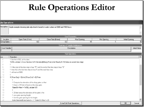
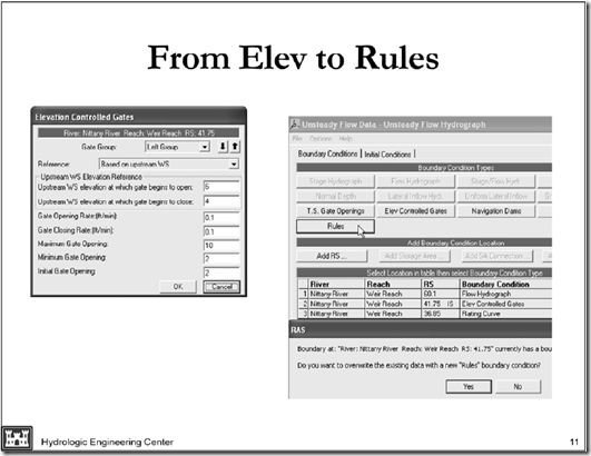
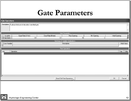
Rules for controlling hydraulic structures can be entered after an inline structure, lateral structure, or storage area connection has been added to the project. From the Unsteady Flow Data editor, add or select the given structure and then click on the Rules button. This will bring up the Gate Rule Operation editor (as shown in the next slide). In the Gate Parameters table at the top of the editor, some initial information can be entered for any gate groups that are in the hydraulic structure.
The Open and Close Rate controls how fast the gates can move. So if, for example, a rule operation required the gate to open one additional foot and the gate opening rate was 0.1 ft/min and the user had selected a one minute time step, it would take ten time steps for the gate to reach the new opening height.
image
The Open and/or Close Rate can be left blank, which means the gate can move to any new setting in a single time step.
The Max and Min Opening will constrain the maximum and minimum gate opening settings. Building on the previous example of opening the gate one additional foot, if the gate was at 3.5 feet and the maximum was set to 4 feet (even though the gate was 6 feet tall), over a five minute period, the gate would open to 4 feet and then stop. If the Max is left blank, then the gate maximum opening is limited only by the height of the gate. If the Min is left blank, then the minimum opening is fully closed (i.e. 0.0).
The Initial Opening provides the first setting for the gate. This opening height will be used during the initial backwater computation. The gate will be left at this setting until it is changed by a rule operation. The Initial Opening is required for all gate groups, if any, in the hydraulic structure and may not be left blank.
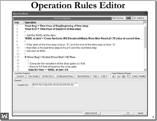
In this example, row 7 is getting the wsel at the dam. Row 13 is checking to see if it is 0600 hours. If it is, then rows 17 and 22 are executed. Row 17 computes a new gate opening elevation for the drop gates. The new elevation is 3.5 feet below the wsel at the dam. Row 22 converts the elevation into an actual gate opening and tells the program to use the new gate opening. The final result is that at 0600 hours the drop gates are adjusted to have 3.5 feet of head on them.
To enter or edit the rule operations, click the Enter/Edit Rule Operations button.
Image_008
image Operation Types:
Comment. Provides a user entered line of text (for documentation only).
New Variable.  Allows the user to create a variable and give it a custom name.
Get Simulation Value. A variable is set equal to a given value in the simulation, such as the flow at a cross section or the time of day.
Set Operation Parameter. Changes the operation of the hydraulic structure, for example, adjusting the gate height or setting a maximum discharge.
Branch (If/Else). Controls which operations are executed on the basis of an If-Then test (e.g., do different gate operation checks based on seasonal considerations).
Math. Performs math operations such as summing flows or averaging water surfaces.
Table. This operation allows the user to enter a table and perform table lookups to get a value.
image
Image_010
A group of rules for one hydraulic structure is referred to as a rule set. At the start of each time step, each rule set is evaluated to check for changes to the operation of the given hydraulic structure. Rule operations are performed from the first (top) rule to the last (bottom) rule. By default, each rule operation is evaluated once. However, branching operations (If/Then/Else, etc) can cause some rule operations to be skipped. No looping or jumping to prior rule operations is allowed. That is (during a given time step), a rule operation may not be performed more than once.
Note: A rule set is only called once during a time step, even if the program iterates during that given time step. (Whatever rules are “in force” at the start of the time step will apply during all of the iterations).
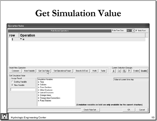
The Get Simulation Value operation provides information about the current state of the model.
In the above example, the wsel at a cross section just upstream of the dam is being retrieved and stored in a variable named “WSEL at dam.”
There are currently seven categories of simulation variables. These are Time, Solution, Cross Section, Inline Structure, Lateral Structure, Storage Areas, and Storage Area Connectors. Clicking on the “+” will expand the list for that category.
For all the variables under Time, the user can select to use the time at the beginning of the time step (default), the end of the time step, or the previous time step.
For the remaining [non-time] variables, the user can select the current value, the value from the previous time, or a “look back” value.
image
Image_012
Clicking the Math operation button creates a math operation as shown. The result of the math operation can be assigned to either a new variable or an existing variable.
The math operation itself is composed of up to four different “expressions.” Each expression that is defined will return a real number. Expressions should be defined from left to right. So if a math operation is composed of two expressions, the left two expressions should be defined
and the right two expressions should be left as “[not set]” (i.e. they should be left blank). If more than one expression is defined, then the user must choose an algebraic connector from the drop down menu between them. The choices are: addition, subtraction, multiplication, and division.
image
Image_014
In order to use a variable in an expression, or store the result into an existing variable, the user selects the variable with a pull down menu, as shown.
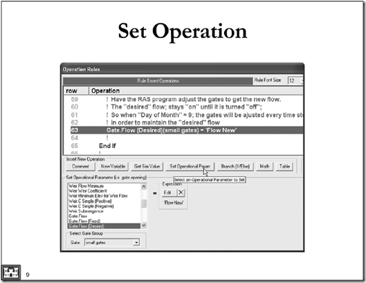
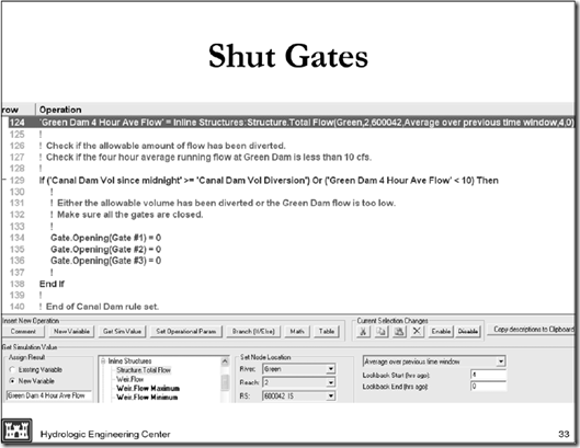
In row 129, there is a two part If/Then. In the first part, the rule operation is checking to see if “Canal Dam Vol since midnight” is greater than or equal to “Canal Dam Vol Diversion.” In the second part, it is checking to see if “Green Dam 4 Hour Ave Flow” is less than 10. Since the two different parts are connected with an “Or,” if either part is true, the expression will be true and rules 134, 135, and 136 will be executed. In more understandable terms, there is a check to see if the maximum amount of water has been diverted, or if the four hour running average flow at Green dam is below 10 cfs. If either is true, then all of the gates will be fully shut (and no more flow will be diverted for the rest of the day). image To control a given aspect of he hydraulic structure, a Set Operational Param rule operation is used. In the example above, rule 63 is setting the “gate flow desired” to the [previously calculated] value of “Flow New.” This will cause the RAS program to adjust the gate settings in order to get the desired flow. (The actual computed flow may be slightly different due to convergence tolerances and changing water surface elevations.)
There are a number of different operational parameters that can be set. In addition to setting the gate opening height or having RAS compute the height to get a desired flow, the user can: set a maximum flow, set a minimum flow, fix a given flow, etc.
image
Image_019
In this simple example, a rule set that is attached to a lateral structure is being used to divert flow from the main river. The diversion is based both on the amount of flow going through a downstream dam and the time of day.
After getting the time of day and the flow at the inline structure, the actual diversion is determined from a lookup table as shown above. So, for instance, if the time is 12 (i.e. 1200) and the flow through the dam is 10,000 cfs, then 1000 cfs will be diverted.
In this example, the user has selected to interpolate. So if, for example, the flow was 11000 at
12 hours, then the flow diverted would be 1100 cfs. Instead, the user could have selected “nearest index value” which would have resulted in 1000 cfs being diverted for a main river flow of 11000. This option could be useful, for instance, if the lookup table was being used to set gate openings that can only be opened in discrete amounts.
Note that in row 13, the flow diversion (‘Flow to Divert’) has been set as a “Total Flow (Fixed)”. This means that the flow being diverted by this lateral structure is being entirely controlled by the rules (and the value from the lookup table). There are no gates and no hydraulic computations (e.g. computed flow over a weir).
image
Image_022
In this, and following, slides, the gate control will be switched from elevation control to a rule set that has the same basic functionality. image The gate opening rates, maximum, minimum and initial gate opening are entered.
Next, the <Enter /Edit Rule Operation> button is clicked.
image
Image_026
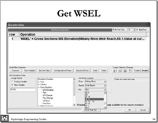
The first rule that is needed is the water surface elevation immediately upstream of the inline structure.
Clicking the <Get Sim Value> button, as shown, will start the creation of the first rule.
image
Image_028
On the left, beneath where it says “Assign Result”, a descriptive variable name should be entered (in this case, WSEL).
Under Simulation Value, the Cross Section tab should be expanded and WS Elevation chosen.
Next, the river station just upstream of the inline structure is selected from the pull down menu.
On the right, the default “Value at current time step” should be left as-is. This gets the water
surface at the start of the timestep. Other choices would get a previous water surface or a
lookback/time-averaged water surface.
image
Image_030
The next step is to add a rule that checks to see if the water surface is high enough that the gates need opening.
Clicking on the <Branch (If/Else)> button, will start the second rule. The If test compares the value of two different “Expressions”. Clicking on <Edit> underneath the Expression on the left will bring up the Edit Rule Expression editor as shown. Clicking on the Variable pull down menu will show all of the variables in the rule data set. In this case there is only one. Selecting the variable WSEL (which is created by rule 1), allows the value of the water surface to be compared to the second expression. Since the water surface is the desired item, the rest of the fields are left blank. (If it was desired, the Variable could be multiplied by a Coefficient, raised to an Exponent, and/or a Constant added.
image
Image_033
For this If test, the check is to see if the water surface is greater than 6.0 feet. Between the two Expression buttons, there is a pull down menu that is used to select the “>” (greater than) operator.
The right Expression is clicked and the number 6 is entered in the Constant field.
image
Image_035
The next rule is to set the gate opening height when the water surface is above 6.0 feet.
Clicking the <Set Operational Param> button will display the menu on the lower left and the
Gate.Opening operation is selected. Under Select Gate Group, the Left Group is selected.
The gate opening is set to 10.0 feet using the expression editor.
image
Image_037
Every If rule must have a corresponding End If. Click the <Branch> button, which initially creates an If rule. Change this rule to an End If by the selecting the End If radial button as shown.

image Another conditional must be created to close the gates when the water surface gets low enough.
The quickest and easiest way to do this is by making a copy of the existing rules (that open the gates), and then editing the copy.
Highlight rules 2 through 4 by clicking on rule 2 and then pressing the down arrow while holding the shift key (shift + down arrow).
Next, click on the Copy button, then move the cursor below row 4 (as if a new rule was to be made using one of the standard Insert New Operation) and then click on the Paste button.
The keyboard shortcuts Ct+X and Ctrl+V, can be used instead of clicking on the copy and paste keys.
Copying existing rules using the Ctrl+X and Ctrl+V shortcuts (and then editing the copy) can save a lot of time and effort.
image
The next step is to edit the just copied rules.
The 6 needs to be changed to a 4 (in the If rule), the operand needs to be changed from a greater than to a lesser than, and the gate opening value needs to be changed from 10 to 2.
image
Image_044
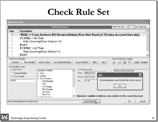
Finally, it is a good idea to click on the <Check Rule Set> button. RAS will check for any basic errors in the rule data set. (For instance, if there is a If rule that does not have a corresponding End If.) If the Check Rule is not performed at this stage, RAS will still perform the check at run time. Errors will generate a message for the user about the problem. The Check Rule button is
a short cut that allows the user to identify problems while the Operation Rule editor is still open.
image
Image_046
In addition to If/Then, the rules also allow for If/Then/Else and If/Then/ElseIf/Else type constructions (as well as nested If/Then statements).
In the above example, the gate opening will be set to 10 if the WSEL is greater than 6.0 feet. Otherwise, the opening will be set to 6 feet if the WSEL is above 5.0 feet. Finally, it will be set to 2 feet if the WSEL is less than 4.0 feet.
If the WSEL is less than or equal to 5 feet, but greater than or equal to 4 feet, the gate opening will not be changed.
image
Image_048
Deciphering (aka debugging) what a complicated rule set is actually doing can be tricky. RAS has a text based output file referred to as the Detailed Log. The operation of each rule in a rule set can be examined on a timestep by timestep basis from this log.
The log output is turned on as shown above.
Image_050 image Every rule that is executed will be shown—as will the result of that rule. The output shown above is taken from the previous rule data set that opens the gate when the WSEL is greater than
6.0 feet.
Rule 1 is executed and the variable WSEL is set to the water surface which is around 6.01 feet.  Rule 2 is executed and this rule is True because the value of the first expression (~6.01) is
greater than the second expression (6.0).  Rule 3 is executed and the gate opening for the Left Group is set to 10 feet. No other rules are executed for this rule data set (for this time step).  Use the find function to locate when things happen. For instance, the string “0002 True” was searched on to find this location in the log file.
Note: having detailed (debug level) output for the rule data set directly available within the
GUI is already on the RAS “wish list”.
image
Image_053
The canal data set (which is included as one of the sample data sets when RAS is installed) provides a good example of the sophisticated operations that are possible with the advanced rule capability.
In this data set, the rules are being used to allow RAS to model a reservoir and a water supply canal in Florida. The Florida water district has a complicated operating agreement that it must conform with.
A reservoir has been modeled as a series of cross sections. A water supply canal leaves the side of the reservoir. This has been modeled with a junction and an inline structure (shown above and red circle) on the diversion canal. The main dam on the reservoir is further downstream (and is not shown on the above graphic).
The flat terrain (river gages suffer backwater effects far upstream of the dam) and the large groundwater flows make measuring inflows to the reservoir difficult. Instead, the inflow to the reservoir is assumed to be equal to the outflow (the outflow from the main dam plus the outflow through the water diversion canal).
The water district’s allowable diversion is based on the previous day’s outflow (midnight to midnight). Additionally, the water district is not allowed to divert water when the outflow from the main dam is too low. (The flow at the main dam is reduced when the reservoir drops too low—so, the water district is, indirectly, prevented from making diversions when the reservoir water surface is low.)
Image_056 image

Rules 3 through 5 create three variables. New variables are most often created with a Math or Get Sim Value operation. However, it is sometimes convinent to have the variable creation be its own rule. Note: the Initial Value = 0 sets the variable equal to 0.0 at the very start of the simulation (the very first time the rule set is called for the first timestep). Afterwards, the variable will keep its value between time steps (e.g., if it equal “5” at the end of the first time the rules set is called, it will equal “5” at the start of the next time). To set it equal to 0.0 at the start of each time step, a Math operation should be used.
Rule 10 gets the length of the time step with a Get Simulation rule. A math operation is then used to compute the length of the time step in seconds.
Rules 16 and 17 get the outflow from the main dam and the diversion canal.
Rules 20 and 21 add the volume of outflow (for this time step) to the current volume. The
“current volume” is the volume of outflow since midnight.

Rules 26 and 27 get the day of the month at the beginning of the time step and the end of the timestep. If the data set is using 15 minute time steps, at some point the beginning of the timestep will be at 11:45pm and the end of the timestep will be at 12:00am. When that happens, the beginning day of month will not equal the end. Beginning might be 5 and ending 6, or beginning could be 31 (or 30 or 28) and the end will be 1 (the first of next month).
Note: The rules use a 24 hour clock, so in the above example, the timestep would actually be at
23:45 and 00:00.
image
Image_059
Rule 31 checks to see if it is midnight. When the timestep starts and ends on different days, it is midnight.
Rule 39 computes the total average outflow for the previous 24 hours (in cfs). Rules 42 and 43 zero out the volume variables for use for the next day.
The methodology for determining the allowable diversion is based on the amount of outflow. No diversion when the flow is less than 100 cfs (rule 47). 10% of the previous days flow when the flow is between 100 and 150. A sliding scale (from 10% to 30%) when the flow is between
150 and 215. 30% for flows between 215 and 1000 and a maximum of 300 cfs (for flows over
1000).
image
Image_061
Up to four separate expressions can be combined into a single Math operation.Image_063
image
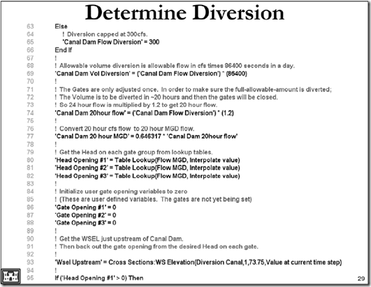
Rule 69 converts the allowable diversion from cfs to a daily volume.
The gates are adjusted at midnight and are left in place until the allowable diversion has taken place. The gate flows are computed so that the diversion will take approximately 20 hours. (If the flow was based on a 24 hour diversion and the gate flow was slightly less than assumed, then the gates would either have to be adjusted or the full, allowable diversion would not take place).
Rule 77 computes the 20 hour flow on a MGD basis.
image
Image_065
The inline structure has three different gate groups (that are used in normal operations). The gates are overflow (drop) gates.
For each gate group, the water district has a table that shows the amount of head that should be on that gate group for a given flow.
Rule 80 computes the amount of head needed on gate group #1 using the lookup table (shown above). The value that goes into the lookup table (input) is determined by the expression editor. In this case it is the “Canal Dam 20 hour MGD” variable (which the first part of the name can just be seen left of the lookup table). The result of the lookup (output) is stored in a new variable, “Head Opening #1”.
image
Image_067
The head on the drop gate is the upstream water surface minus the gate opening height minus
the invert elevation of the gate. Rearranging, gives the gate opening to be equal to the head plus the invert minus the upstream water surface as computed in rule 100.
Rule 100 computes the desired gate opening.
Rule 105 actually sets the gate opening to the value that was computed by rule 100.
The computation for the gate opening involves two different variables (Head and WSEL), which meant that two different “Expressions” had to be used. The Set Gate Opening command only has a one Expression. So a Math operation was used (which can have up to 4 different variables/expression) in rule 100.
Image_069
image   image
There are two different triggers for shutting the gates:
One trigger is the first part of rule 129. It checks to see if the allowable volume of water has been diverted. If it has, then rules 134-136 make sure all the gates are closed.
The other trigger is based on the outflow from Green dam. When the flow at Green dam is below 10 cfs, the water district must stop diverting water. (This only happens at low reservoir levels.) However, it is possible for the reported flow at Green dam to briefly drop below 10 cfs, either because of a switch in gate operations or because of a “missing value” from the remote data operation. To accommodate this, the water district does not have to stop the diversion until the average flow over 4 hours has dropped below 10 cfs.
Rule 124 computes a running, 4 hour average of the flow from Green dam. Looking at the lower right of the above screen shot, the Lookback period is from 4 hours ago to the current times step (0 hours ago).
The second part of rule 129 checks if this 4 hour average is below 10 cfs. If it is, all of the gates are closed.
image
Image_072
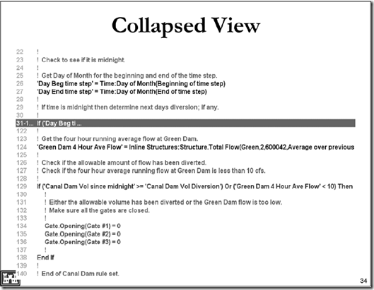
The rules between an If/Then and it corresponding End If can be collapsed and/or expanded. This is done by clicking on the “+/-” to the left of the row number. This option can make viewing complicated data sets easier. (The rules are still active.) All of the rules that are involved in the once daily computations (at midnight) have been collapsed, above.