Written by Aaron A. Lee | WEST Consultants
Copyright © RASModel.com. 2011. All rights reserved.
By using the Mixed Flow Regime option for Unsteady Flow Analysis, RAS can better handle transitions from subcritical to supercritical flow. This option should be utilized only after determining that a mixed flow situation exists, which requires judgment from the modeler. One application where this could be particularly useful is dam breach modeling, or any other extreme and flashy flood event. Even though a model is stable there may still be small errors in the solution (caused by max. iterations). The Local Partial Inertia (LPI) factor may eliminate or reduce these errors, particularly if they occur when the Froude number is near 1. Figure 1 shows the Unsteady Flow Analysis window with the Mixed Flow Regime option selected. This post will focus on the LPI Filter, which is enabled when Mixed Flow Regime is selected by the modeler.
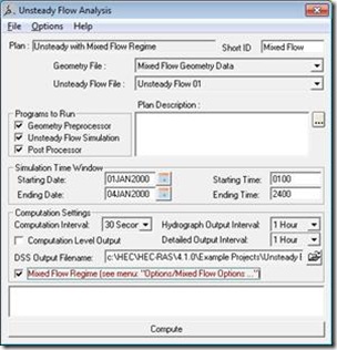
Figure 1. Unsteady Flow Analysis Window
Once the Mixed Flow Regime option is selected, additional settings can be adjusted to help stabilize the model. Navigate to Options, Mixed Flow Options. This window, shown in Figure 2, allows the user to adjust two inputs for the LPI factor.
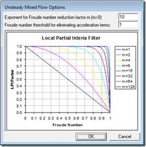
Figure 2. Mixed Flow Options Window
For the unsteady flow computation scheme, RAS accounts for a local acceleration and convective acceleration (inertial terms) through the St. Venant equation of Conservation of Momentum. The St. Venant equations, and by extension, HEC-RAS, are designed to work best in gradually varied flow. Transitions from supercritical to subcritical flow (hydraulic jump), and to a lesser extent subcritical flow to supercritical flow, are rapidly varied flow situations. These are not gradual changes, in the hydraulic sense. Near critical depth (Froude number approaching 1) the convective acceleration terms can change very rapidly over a short distance (think of a hydraulic jump) and can lead to oscillations in the solution. These oscillations tend to grow larger until the solution goes completely unstable (HEC, 2010). The LPI factor systematically reduces these inertial terms to dampen the oscillations, helping to stabilize the model. The user can influence the magnitude of reduction by varying the two inputs in Figure 2.
The first input, m, is the exponent for Froude number reduction factor. Its default value is 10 and ranges from 1 to 128. Adjusting m will change the shape of the curve on Figure 2, thus influencing the rate of reduction of the inertial terms. You can see that by making m smaller there is an earlier and more direct reduction in the inertial terms, with respect to the Froude number. Increasing m can make the model more accurate but increases the likelihood of numerical instability.
The second input, FT, is the Froude number threshold at which the LPI factor is set to zero. In other words, if the calculated Froude number at the current cross-section is larger than FT the inertial terms will be eliminated from the computations at that cross-section for the current computational time step. The default value is 1. Making FT smaller will improve the stability of the model, but will also reduce the accuracy. A larger FT can make the model more accurate, but increases the likelihood of numerical instability as the inertial terms will be more sensitive to fluctuations in Froude number.
A good place to start is to run the simulation with the default values
and see what the profile looks like. For this flume example, the model ran without reporting any maximum water surface errors. The profile for the default LPI inputs is shown in Figure 3.
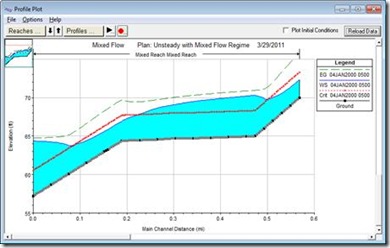
Figure 3. Profile Plot, Default Values
Next, a value of 1.6 was chosen for FT. This simulation yielded small maximum water surface errors, but had maximum iterations at various locations. The value of m was left unchanged. Figure 4 shows the results.
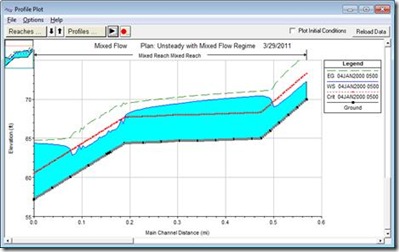
Figure 4. Profile Plot, Increased Froude Number Elimination Threshold
Even though the errors were small, instabilities could be seen in the downstream end. Notice the instabilities around the transitions between the flow regimes. The value of m was reduced from the default of 10 to 7 in order to improve the stability of the model. Figure 5 shows the profile for reduced m and increased FT. The modeler should choose the largest values of m and FT that produce a stable model. However, check the results to make sure that the output is reasonable. Notice how the transitions between flow regimes are much better defined in Figure 5 then the default setup shown in Figure 3. That’s because the default LPI parameters (m = 10 and FT = 1) provide dampening of the results. Though Figure 3 looks very stable (and it is), Figure 5 (m = 7 and FT = 1.6) is both stable and (by my engineering judgment) more accurate. Also, notice how the slight increase in energy (green dashed line) is less in Figure 5 versus Figure 3. An increase in the energy elevation in the direction of flow is an indication of error in most cases. Further adjustment of the LPI parameters may help to eliminate the error in the energy grade line, while still producing a stable solution.
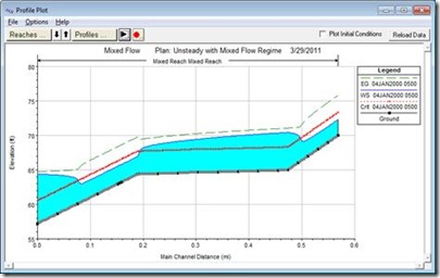
Figure 5. Profile Plot, Increased Froude Number Elimination Threshold and Decreased Exponent ,m
Copyright © RASModel.com. 2011. All rights reserved.
By using the Mixed Flow Regime option for Unsteady Flow Analysis, RAS can better handle transitions from subcritical to supercritical flow. This option should be utilized only after determining that a mixed flow situation exists, which requires judgment from the modeler. One application where this could be particularly useful is dam breach modeling, or any other extreme and flashy flood event. Even though a model is stable there may still be small errors in the solution (caused by max. iterations). The Local Partial Inertia (LPI) factor may eliminate or reduce these errors, particularly if they occur when the Froude number is near 1. Figure 1 shows the Unsteady Flow Analysis window with the Mixed Flow Regime option selected. This post will focus on the LPI Filter, which is enabled when Mixed Flow Regime is selected by the modeler.

Figure 1. Unsteady Flow Analysis Window
Once the Mixed Flow Regime option is selected, additional settings can be adjusted to help stabilize the model. Navigate to Options, Mixed Flow Options. This window, shown in Figure 2, allows the user to adjust two inputs for the LPI factor.

Figure 2. Mixed Flow Options Window
For the unsteady flow computation scheme, RAS accounts for a local acceleration and convective acceleration (inertial terms) through the St. Venant equation of Conservation of Momentum. The St. Venant equations, and by extension, HEC-RAS, are designed to work best in gradually varied flow. Transitions from supercritical to subcritical flow (hydraulic jump), and to a lesser extent subcritical flow to supercritical flow, are rapidly varied flow situations. These are not gradual changes, in the hydraulic sense. Near critical depth (Froude number approaching 1) the convective acceleration terms can change very rapidly over a short distance (think of a hydraulic jump) and can lead to oscillations in the solution. These oscillations tend to grow larger until the solution goes completely unstable (HEC, 2010). The LPI factor systematically reduces these inertial terms to dampen the oscillations, helping to stabilize the model. The user can influence the magnitude of reduction by varying the two inputs in Figure 2.
The first input, m, is the exponent for Froude number reduction factor. Its default value is 10 and ranges from 1 to 128. Adjusting m will change the shape of the curve on Figure 2, thus influencing the rate of reduction of the inertial terms. You can see that by making m smaller there is an earlier and more direct reduction in the inertial terms, with respect to the Froude number. Increasing m can make the model more accurate but increases the likelihood of numerical instability.
The second input, FT, is the Froude number threshold at which the LPI factor is set to zero. In other words, if the calculated Froude number at the current cross-section is larger than FT the inertial terms will be eliminated from the computations at that cross-section for the current computational time step. The default value is 1. Making FT smaller will improve the stability of the model, but will also reduce the accuracy. A larger FT can make the model more accurate, but increases the likelihood of numerical instability as the inertial terms will be more sensitive to fluctuations in Froude number.
A good place to start is to run the simulation with the default values
Technorati Tags: HEC-RAS,RAS,Mixed Flow,LPI Method,Unsteady Flow,Supercritical,Subcritical,Hydraulic Jump,Froude,Water Surface Profile,Dam Breach,Dam Break,Flood,Numerical Model,St. Venant
and see what the profile looks like. For this flume example, the model ran without reporting any maximum water surface errors. The profile for the default LPI inputs is shown in Figure 3.

Figure 3. Profile Plot, Default Values
Next, a value of 1.6 was chosen for FT. This simulation yielded small maximum water surface errors, but had maximum iterations at various locations. The value of m was left unchanged. Figure 4 shows the results.

Figure 4. Profile Plot, Increased Froude Number Elimination Threshold
Even though the errors were small, instabilities could be seen in the downstream end. Notice the instabilities around the transitions between the flow regimes. The value of m was reduced from the default of 10 to 7 in order to improve the stability of the model. Figure 5 shows the profile for reduced m and increased FT. The modeler should choose the largest values of m and FT that produce a stable model. However, check the results to make sure that the output is reasonable. Notice how the transitions between flow regimes are much better defined in Figure 5 then the default setup shown in Figure 3. That’s because the default LPI parameters (m = 10 and FT = 1) provide dampening of the results. Though Figure 3 looks very stable (and it is), Figure 5 (m = 7 and FT = 1.6) is both stable and (by my engineering judgment) more accurate. Also, notice how the slight increase in energy (green dashed line) is less in Figure 5 versus Figure 3. An increase in the energy elevation in the direction of flow is an indication of error in most cases. Further adjustment of the LPI parameters may help to eliminate the error in the energy grade line, while still producing a stable solution.

Figure 5. Profile Plot, Increased Froude Number Elimination Threshold and Decreased Exponent ,m

Hi,
ReplyDeleteIs it possible to apply the mixed flow option to some reaches and not to others? I am currently modelling a dam breach that flows from a steep small channel and into a large river that is relatively flat. When the mixed flow options are turned off the flat large river produces nice results but the steep channel's flow is not correct. When it is turned on (default), the steep channel produces good results. Playing around with the LPI does not seem to be helping.
Any thoughts?
Thanks,
Sarah
Hi Sarah-
ReplyDeleteWhen you turn on the mixed flow option, it is applied everywhere and at every timestep in your model. However, there will be minimal to no affect when and where Froude Numbers are low, depending on how you set your LPI controls.
It could be an HTAB parameter problem. Make sure that in your steep reach, your HTAB computations start at the invert of each cross section and that there is good resolution (i.e. a lot of computation points). See this blog post for more info on HTAB parameters:
http://hecrasmodel.blogspot.com/2011/03/more-on-htab-parameters.html
Hi.I am Urban Planner & GIS expert by profession..My boss assigned project regarding Glacial lake outburst floods & use of HECRAS to show its effects onn near settlements...I am came up with BREACH model for such cases & HECRAS..can any one assist me, b/c it will help many poor people to cope with climate change & its impacts..
ReplyDeleteMasood Ali from Gilgit
Mr. Ali-
ReplyDeleteWhat kind of help are you looking for? You can email me at cgoodell@westconsultants.com if you'd like a more efficient line of communication.
Chris
Hi,
ReplyDeleteI'm now modelling a channel, which's bed slope is mostly big, and in some parts covered. The steady analysis gave a well solution, via mixed flow calculation, but I can't stabilize the same model for unsteady calculations. I followed tips from Your posts, which worked well before, but now the unstable state of the calculation stays incredibly huge. I interpolated the x's within the whole reach, the lower boundary is normal depth in both calculations, the upper one is flow, and flow hydrograph. I tried to follow Your advice here by changing the reduction factor and FT, but the ammount of errors in the calculation hardly changed, whatever I tried to change. What else could I do, or had forgot?
Thanks,
Gergely
Hey Gergely, Send me a debug report zip file of your model data files (go to this link if you don't know how to do that). http://hecrasmodel.blogspot.com/2008/12/hec-ras-debug-report.html
DeleteI'll take a quick look to see if I can figure it out.
cgoodell@westconsultants.com
Thanks for the fast response Chris, the report is on it's way!
DeleteHello, I have a question...
ReplyDeleteI’m modelling sediment transport (quasi-steady flow)
After running the model the Froude Number is equal or less than 1 in all the river, there is not super-critical flow.
In Sediment transport simulation there is not the MIXED FLOW option. You know something about this?
I performed the steady and unsteady flow too, the results show that in these points the river has supercritical flow (froude number>>1). I don't understand why in quasi-steady froude are equal or less than 1.
Thanks...
I believe that sediment transport does not support supercritical flow in the current version. Where you see Froude Number equal to 1 is likely a place where it wants to be supercritical, but since RAS will not compute a supercritical result for sediment computations, it defaults to critical depth (Froude number = 1).
DeleteThanks Chris, i couldnt believe it, but sediment transport does not support supercritical flow. The version 5 beta neither...
ReplyDeleteHi, when i running unsteady flow, i've some problem like "HTab Parameter for starting elevation is lower than lowest elevation in the cross section main channel". what should i do ?
ReplyDeleteThis can happen if you do some manual changes the the invert of one or more cross sections. Easy to fix. Go the the HTAB Param. button in the geometry editor. Make sure you have All River selected. Then highlight the entire column with the header "Starting El". Then click the button at the top that says "Copy Invert". That should fix it.
DeleteHello,
ReplyDeleteI have a question that concerns the mixed flow regime for a steady flow analysis. I'm modeling a steep channel which contains a very narrow and flat section in the middle. A hydraulic jump occurs right before that section and a few meters downstream the flow changes back to supercritical. Now the computation works fine for all of the cross sections (interpolated or not) except for the one cross section where the flow changes from subcritical to supercritical. There I get the warning that the energy equation could not be balanced and that the program defaulted to critical depth. When i modified the Manning's values so the change of flow would take place at another cross section that type of warning now appeared for the other xs. So I don't think that my cross section data is bad and I'm sure I interpolated properly.
Is there something I could do?
Thanking you in anticipation, greetings from Germany
A couple things about supercritical flow. First, you typically need much closer spaced cross sections. I would try doing even more interpolation. Also, make sure you are using the suggested contraction and expansion coefficients for supercritical flow (0.01 and 0.03 as opposed to 0.1 and 0.3 for subcritical). Finally, at the contraction and expansion, make sure you have your ineffective flow areas properly defined. If you believe there will be flow separation as flow contracts and expands, there needs to be ineffective flow areas.
DeleteHello i simulate a canal there is a box culvert in the mont of the canal when I put the flow and run the simulation the canal and the culvret are submerged and there is a problem of flood so my question wich regim of flow i should use if Subcrit. Supercrit, mixed please help me
ReplyDeleteIf steady flow, and you're not sure of the regime, try mixed flow. If it is indeed all sub critical, then you'll see that. Note that for unsteady flow, RAS will compute mixed flow automatically, whether you check the mixed flow box or not. Checking the mixed flow box for unsteady just adds stability to the computations when you are near or transitioning through critical depth.
DeleteHello, I need to simulate flood in steep river (slope 15%) in 2D. 2D is not problem, but there are some bridges in the area. I wanted to simulate bridges in 1D and then use rating curves for 2D model to simulate these bridges. Problem is that there is a lot of warnings in 1D model and it is not computing right. I think it is caused by steep slope. Solution could be 2D model with bridges modeled as a gates, but there is no data for calibration of bridges flow. So what do you recommend to simulate bridges in steep rivers please?
ReplyDeleteLots of close cross sections, lots of resolution with your bridge htabs, try exploring other bridge modeling approaches.
DeleteHello Chris.
ReplyDeleteI would like to make a question just for clarification. Is the LPI in Hec-Ras the method for shock wave capturing (like for instance the TVD solver in Flood Modeller software)? Does Ras has any specific solver for this occasions (e.g. Dam Breach)?
Thank you so much Chris in advance. Keep on teaching us!! : )
Regards,
Ioannis
Hi Ioannis-
DeleteI don't know about the TVD solver in Flood Modeller, but the LPI reduction factor dampens the "hyperactive" acceleration terms in the St Venant equation when you are close to critical depth. It is nearly always needed for dam breach modeling.